Vibrational Pooling and Constrained Equilibration on Surfaces

(1)

Vibrational Pooling and Constrained Equilibration on

Surfaces

Thesis by

E. T. D. Boney

In Partial Fulfillment of the Requirements

for the Degree of

Doctor of Philosophy

California Institute of Technology

Pasadena, California

2014

(2)

c 2014

E. T. D. Boney

(3)

(4)

Acknowledgments

Who knows how long it took Mike Slackenerny? After seven years, I appear to have finally done

enough to graduate.

My supporting cast of characters is wide, and I do not thank them enough. First, thanks go to

my wife Susanna, whose support has helped me through the long laborious years. I love you, Mrs.

Dooley Boney; thank you for all the bike rides to concerts, across the Black Rock Desert, and all

the sunsets down at the Japes.

Secondly, I must thank my family for raising me with an appreciation of science and knowledge,

and raising me safe and sound as well. Mom and dad, thank you.

Scientifically, I have the most debt to my advisor, Rudy Marcus, and I will spend a few winding

paragraphs thanking him. I came to Caltech because Rudy had not changed his research philosophy

his whole career: theory guided first and foremost by interesting experiments. If you cannot explain

what people are interested in, then what is your theory good for?

His philosophy is unique, and in my work with him, Rudy has never given in to my urge to

publish prematurely. We did not explain experimental results that wound up retracted with my first

big paper; this prudence was his, not mine. When that retraction wound up wasting about four

years of mean-field work on H:Si(111) and other surfaces, his focus on experiments guided us.

In the end, we found some cool fluorescence results from the late 1980s and early 1990s, and

explained vibrational population inversion on surfaces in a way that has previously been done in

gases by Treanor. Such inversion could change every sort of measurement at surfaces, not just old

fluorescence experiments, from STM and AFM to SFG and SHG, there is now a new possibility

besides defect, bridge, dimer or trimer that demands consideration: the vibrational pool! Because

of his inkling that we had more to discover, we were able to do unifying work between the gas phase

and interfaces that I find very philosophically satisfying in a way that has nothing, and everything,

to do with experiment.

Other advice of his that cannot be ignored by anyone searching here for his wisdom is to know

the literature. Because we want to be guided by experimental results, we have to find and correctly

interpret the existing data as soon as we can. If we reach the bounds of the literature and have not

(5)

with. Along those lines, I owe a great debt to Huan-Cheng Chang, Hugh Richardson, George Ewing,

Chifuru Noda, Steven Corcelli, Phillippe Guyot-Sionnest, and John Tully, who did the bulk of the

experimental and theoretical work underpinning my thesis. Without them, I would not have had

anything to do. I owe a special debt to collaborator Jim Lyons, who developed the isotope mixing

code and edited the chapter on self-shielding.

Besides advice from Rudy, I also benefited greatly from the comments of my committee, and

thank them now by name for their general wisdom as well as cumulative specific advice: Rob

Phillips, Aron Kupperman, Tom Miller, and Jim Heath.

Furthermore, in my time at Caltech, I have had the opportunity to know unique individuals

that have shaped my way of thinking about the world in positive and permanent ways. They are,

in no particular order (lots of Doctors, so forget the honorifics): Nima Ghaderi, Oliver Eslinger,

Jorge Cham, Jonny Haug, Allyce Ozarski, Lauren Lebon, Nicolas LaCasse, Sanza Kazadi, Andy

Downard, Glenn Garrett, Michael Shearn, Dan Riley, Anna Beck, Faisal Amlani, Paul Minor, Jerry

Maine, Alex Romero, Vahe Gabuchian, Drew Kennedy, Meg Rosenberg, Meher Ayalasomayajula,

Yousung Jung, Maksym Kryvohuz, Nick Agich, Josh Moorhead, J. P. Chism, Brian Duistermars,

Young-In Oh, Ronnie Bryan, Artur Menzeleev, Jason Goodpaster, Rosemary Rohde, Scott Kelber,

Geo↵rey Lovely, Travis Essl, Chris Dae✏er, Ian Tonks, Nathan Hodas, Wei-Chen Chen, Zhaoyan Zhu, Yun-Hua Hong, and Sandor Volkan-Kacso. I also have had several cats whose company I have

enjoyed thoroughly, despite my cat allergies: Mrs. Kitty, LadyBird Johnson, Trash Cat, and Flea,

you were all good kitties.

At MIT, I developed my love of theoretical physical science combined with video games,

au-tomaton programming competitions, ten consecutive Mystery Hunts, Hoegaarden, and philosophical

musings, thanks in large parts to MIT dorm mates who remain some of my closest friends:

Den-nis Wei, Billy Waldman, Sheel Dandekar, Jon Ursprung, Downtown Twarog, Robert Jason Harris,

Gabe Durazo, and Michael Mooney. I may stand on the shoulders of great scientists I’ll never meet

in my research, but I stood with you in reality, contemplating the wonders of the universe from a

revolutionary war park in the dead of night.

Finally, it would be remiss of me not to thank the ARO, ONR, and NSF for their financial

(6)

Abstract

In this thesis, we provide a statistical theory for the vibrational pooling and fluorescence time

dependence observed in infrared laser excitation of CO on an NaCl surface. The pooling is seen

in experiment and in computer simulations. In the theory, we assume a rapid equilibration of the

quanta in the substrate and minimize the free energy subject to the constraint at any time t of a fixed number of vibrational quantaN(t). At low incident intensity, the distribution is limited to one-quantum exchanges with the solid and so the Debye frequency of the solid plays a key role in limiting

the range of this one-quantum domain. The resulting inverted vibrational equilibrium population

depends only on fundamental parameters of the oscillator (!e and !e e) and the surface (!D and

T). Possible applications and relation to the Treanor gas phase treatment are discussed. Unlike the solid phase system, the gas phase system has no Debye-constraining maximum. We discuss the

possible distributions for arbitrary N-conserving diatom-surface pairs, and include application to H:Si(111) as an example.

Computations are presented to describe and analyze the high levels of infrared laser-induced

vibrational excitation of a monolayer of absorbed 13_{CO on a NaCl(100) surface. The calculations}

confirm that, for situations where the Debye frequency limitedn domain restriction approximately holds, the vibrational state population deviates from a Boltzmann population linearly inn. Nonethe-less, the full kinetic calculation is necessary to capture the result in detail.

We discuss the one-to-one relationship between N and and the examine the state space of the

new distribution function for varied . We derive the Free Energy,F =N kT kT ln(PPn), and

e↵ective chemical potential, µn ⇡ kT, for the vibrational pool. We also find the anti correlation

of neighbor vibrations leads to an emergent correlation that appears to extend further than nearest

(7)

c 2014

E. T. D. Boney

(8)

List of Figures

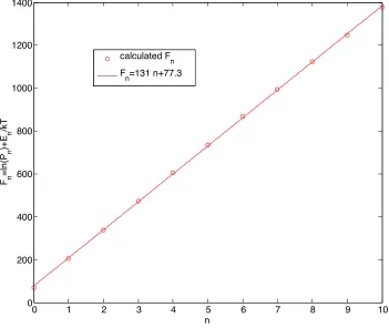
1.1 The fit for the parameter, . The representative pool is derived from monolayer

popu-lations, calculated elsewhere by kinetic Monte Carlo,1_{as the slope of}_ln₍_P

n) +En/kT,

vs. n, the vibrational state. For the Pn calculated near the end of a pulse of the

conditions of the previous monolayer experiment,2 _{= 131. . . .} ₈

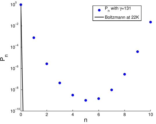
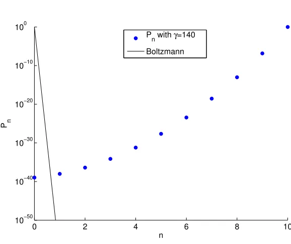
1.2 This figure shows thePn from Eq. 1.4 compared to the Boltzmann distribution at 22K

for = 131. . . 8

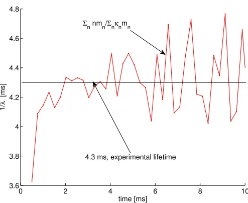
1.3 Calculated 1/ (t) versus time, compared with the single exponential observation. . . 10 1.4 The total overtone fluorescence decay (circles computed) matches experiment (solid

single exponential with⌧=4.3 ms). . . 10

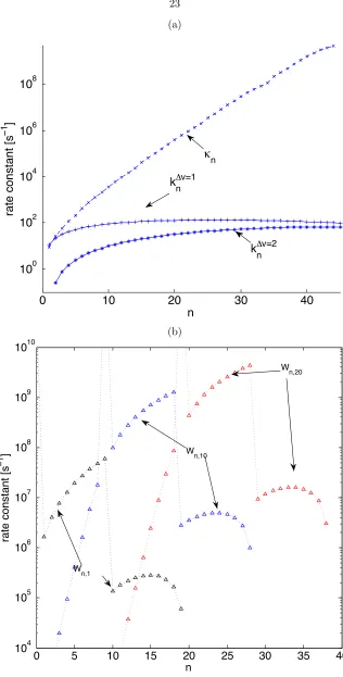
2.1 Comparison of relevant rate constants: (a) first-order rate constants of relaxation (n), fluorescence (k v=1

n ) and overtone fluorescence(knv=2) (b) second-order rate constants

of pooling (Wn,mp form=1,10 and 20). The second order e↵ect of pooling to state n

from anm= 1 state which requires an additional phonon to transfer to n 10, and soW_10,1p _⇡10 3_Wp

9,1. As second order rate constants, the pooling and depooling rate

constants should be multiplied by a conditional probability if one wishes to compare

with the first order rate constants, leading to units [s 1_{per unit conditional probability}

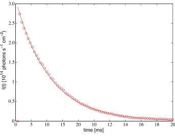
P(m_|n)], as discussed in Chapter Appendix B. . . 23 2.2 The total overtone fluorescence decay (circles computed) matches experiment (solid

single exponential,I(t) =I(0)exp( t/⌧), with time constant⌧=4.3 ms). . . 24 2.3 The vibrational population 6µsfollowing beginning of pulse (near end of lasing). . . 24 2.4 The vibrational population 1 ms following the beginning of lasing. . . 25

2.5 The fit of the computed results to the theory-based expression permits the evaluation

of statistical parameter = 130, from the slope of the linear fit on the restricted n

domain. A typical result forPnafter 4 ms following monolayer excitation is displayed,

(11)

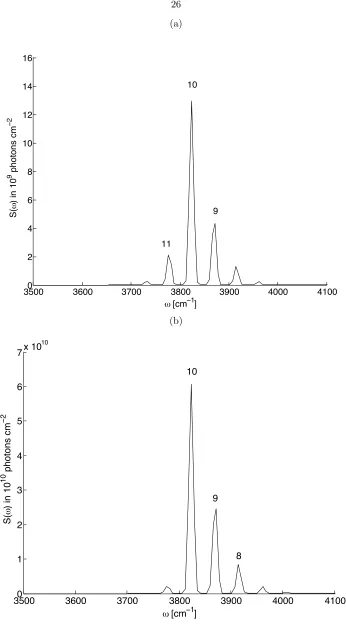
2.6 The theoretical dispersed fluorescence (assuming perfect collection efficiency) for a monolayer under the experimental monolayer lasing conditions (kabs=9 x 104s 1),

in-tegrated over a (a) 1 ms and (b) 20 ms period after the beginning of lasing.2 _The

temporal integration was calculated trapezoidally fromPn(t) at 79 time points spread

equally over the length of calculation. . . 26

2.7 The theoretical dispersed fluorescence (assuming perfect collection efficiency) after (a) 1 ms and (b) 8 ms following CLIO excitation of a monolayer (averaged over a macro pulse

for the highest fluence currently available at that wavelength, kabs,CLIO= 5 x107s 1

for 8µs, or 20 mJ). We note that, in (a), the appearance of a tiny higher nshoulder around n = 22 (which is even more pronounced as a relative peak at shorter times, not shown), but that the signal on the ms timescale is overwhelmed by fluorescence

from lowernand the distribution becomes the same as that for the monolayer under continued observation. . . 27

2.8 Snapshots of the theoretical dispersed fluorescence for a monolayer under the

exper-imental monolayer lasing conditions (kabs=9 x 104s 1). The snapshots given are (a)

1 µs between 77 and 78 µs following beginning of excitation and (b) 12.7 µs period ending 1 ms after the beginning of lasing, representative of the di↵erence in results at di↵erent temporal resolutions of collection. . . 28 2.9 The vibrational population of the surface for a single trajectory at the conclusion

of a CLIO FEL pulse (figure (a), 8 µs excitation) and 1 ms thereafter (figure (b),

kabs,CLIO = 5 x107s 1 for 8 µs excitation for both). For (a), the legend is:

n=0-black, 10-red, 20-orange, 25-yellow, 32-white, highest level. For (b) : n=0-n=0-black, 5-red,

10-yellow, 12-white, highest level. . . 29

3.1 This figure shows the formation ofP2, notingP1,ss⇡0.5 . . . 31

3.2 This figure shows N vs. for the domain restricted theory. . . 32

3.3 This figure shows thePn compared to the Boltzmann distribution at 22K for = 130. 33

3.4 This figure shows thePn compared to the Boltzmann distribution at 22K for = 125. 33

(12)

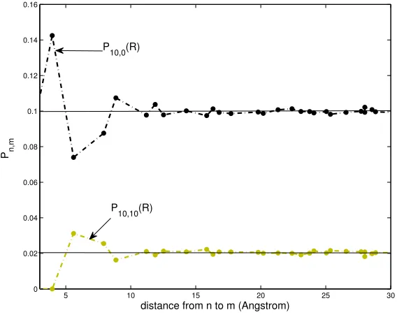
3.6 The vibrational pairwise population 1 ms following the beginning of lasing, compared

with the mean-field expectation of the pair considered, the dashed lines are guides for

the eye: (black)-P10,0, the pairwise probability of an= 10 state next to an= 0 state

(orange)-P10,10, the pairwise probability of an= 10 state next to an= 10 state (note

complete anti-correlation of nearest neighbors). The mean field result for P10,0 and

P10,10 are given by the horizontal lines. Note that, for neighbors, mean-field is a bad

approximation, but for R >> R0, the nearest neighbor distance of 3.96 Angstroms,

mean-field is recovered. . . 35

3.7 In this figure, we see F vs. N, and see the chemical potential (slope) is 2120 cm 1_. From kT in our prior work, we had estimated 1960 cm 1based on from the domain restricted theory. . . 37

3.8 The fit of N kT for 20 ms following Monolayer lasing.2;1;3 _{. . . .} ₃₇

3.9 The fit of N kT for 30 ms following CLIO lasing.3 _{. . . .} ₃₈

4.1 The fit to the experimental loss ofP1,4 1= 1/(5x10 9) s 1 . . . 42

4.2 ThePn vs. n 1.9 ns after lasing with prior conditions.4 . . . 43

4.3 Snapshots of the evolution ofH2from a 50x50 surface under FEL excitation: (a) after 100 ns (b)after 500 ns (c) after 1µs (d) halfway through lasing. We note that the colors indicate black forn = 0 white for n= 21 in (b)-(d), with n= 21, outside the n= 1 20 domain, used to mark the sites that have evolved o↵the surface by associative desorption (white). While we are unable to render the 111 surface (a hexagonal lattice), the square lattice connectivity in figures shown includes diagonals up and to the right and down and to the left of each site, e↵ectively giving 6 neighbors of equal distance. Thus we see diagonally desorbed molecules on the square lattice representation of the 111 surface. . . 44

4.4 Yield ofH2 after a single macropulse vs. Power of macropulse, assuming fast-pooling (calculations shown forµ0 = 1e). . . 45

5.1 A visual representation of the Aikawa-Herbst model. The colors indicate the number densities of molecular hydrogen (red-highest, yellow-medium high, green-medium low, blue- lowest). The arrows in the negative z-direction indicate the direction of incident intensity. The spirals at large R are representative of vertical mixing. Their amplitude indicates the strength of the mixing. Reproduced with permission.5 _{. . . .} ₅₀

(13)

5.4 The synthetic 12_C16_{O spectrum calculated at 50K (black), 300K (red), and 1500K}

(blue). The 50K and 1500K spectra have been shifted -/+0.5 nm respectively for

clarity. The ratio of maxima is approximately 12:4:1. . . 56

5.5 The spectra for the X1_⌃+

g(0) - E1⇧(1) transition of 12C16O,12C17O, and 12C18O at

1500 K . . . 56

5.6 The bandhead in the12_C18_{O spectrum at 1500 K . . . .} ₅₇

5.7 Evidence of a bandhead. This graph shows a bandhead between the 66th and 67th

rotational state for12_C18_{O. . . .} ₅₇

5.8 3-isotope plot at 30 AU with temperature dependent CO cross sections. H2absorption

by shielding function.7. . . 60

5.9 The three isotopomers of12_Cx_{O with a fictitiously high natural linewidth are compared. 61}

5.10 (a)12_C17_{O, (b)}12_C16_{O, and (c)} 12_C18_{O cross section (red) with overlay of H}

2

trans-mission (black). Q-branch of C17_{O coincides with H}

2 transmission feature causing the

vertical 3-isotope trajectory at high temperatures. . . 62

5.11 3-isotope plot with H2 absorption cross sections at 0.035 AU, 0.87 AU, and 30 AU at

(14)

List of Tables

2.1 The calculation times and results for a single trajectory on a 100x100 grid with three

di↵erent resonant rate conditions 1ms following monolayer excitation. They each have relative peaks atn= 10, not shown. . . 18 5.1 Molecular Constants for the various isotopomers of CO in the X1_S

g ground state. All

values given in cm 1_{. Note that e-parity is used for the P and R branches and f-parity}

is used for the Q branch. . . 51

5.2 Molecular Constants for the various isotopomers of CO in the E1_{P excited state. All}

values given in cm 1_{. Note that e-parity is used for the P and R branches and f-parity}

is used for the Q branch. . . 51

(15)

Bibliography

[1] E. T. D. Boney and R. A. Marcus, J Chem Phys, 139, 124107 (2013).

[2] H.-C. Chang and G. E. Ewing, Phys. Rev. Lett.,65, 2125 (1990).

[3] E. T. D. Boney and R. A. Marcus, J Chem Phys (accepted, A13.08.0077).

[4] P. Guyot-Sionnest, P. Dumas, and Y. J. Chabal, J. Electron Spectrosc. Relat. Phenom.,54/55,

27 (1990).

[5] Lyons, J. R., personal communication.

[6] G. Stark, P. L. Smith, K. Ito, and K. Yoshino, Astrophys. J.,395, 705 (1992).

[7] S. R. McCandliss, Pub. Astron. Soc. Pac.,115, 651 (2003).

[8] M. Eidelsberg, J. J. Benayoun, Y. Viala, and F. Rostas, Astron. and Astrophy. Supplement

Series,90, 231 (1991).

[9] S. A. Corcelli and J. C. Tully, J Phys Chem A,106, 10849 (2002).

[10] S. A. Corcelli and J. C. Tully, J. Chem. Phys.,116(2002).

[11] H.-C. Chang and G. E. Ewing, J Chem. Phys.,94, 7635 (1990).

[12] H.-C. Chang and G. E. Ewing, J Chem. Phys.,92, 7635 (1990).

[13] C. E. Treanor, J. W. Rich, and R. G. Rehm, J. Chem. Phys.,48, 1798 (1968).

[14] D. McQuarrie,Statistical Mechanics (University Science Books, 2000).

[15] C. Kittel,Introduction to Solid State Physics (8th _ed.) _{(John Wiley & Sons, 2004).}

[16] P. Guyot-Sionnest, Phys. Rev. Lett.,67(1991).

[17] I. H. Bachir, R. Charneau, and H. Dubost, Chem. Phys.,177, 675 (1993).

[18] H. Gai and G. A. Voth, J. Chem. Phys.,99(1993).

(16)

[20] Z. Liu, L. C. Feldman, N. H. Tolk, Z. Zhang, and P. I. Cohen, Science,312, 1024 (2006).

[21] H.-C. Chang, C. Noda, and G. E. Ewing, J. Vac. Sci. Tech.,8, 2644 (1990).

[22] H.-C. Chang, H. H. Richardson, and G. E. Ewing, J Chem. Phys.,89, 7561 (1988).

[23] H.-C. Chang and G. E. Ewing, Chem. Phys.,139, 55 (1989).

[24] K. A. Fichthorn and W. H. Weinberg, J. Chem. Phys.,95, 1090 (1991).

[25] L. Aleese, A. Simon, T. McMahon, J.-M. Ortega, D. Scuderi, J. Lemaire, and P. Maitre,

International Journal of Mass Spectrometry,249-250, 14 (2006).

[26] D. S. Anex and G. E. Ewing, J. Phys. Chem.,90, 1604 (1986).

[27] H.-C.Chang, personal communication.

[28] P. F. Bernath,Spectra of Atoms and Molecules (Oxford University Press, 2005).

[29] J. A. C. Gallas, Phys. Rev. A.,21, 1829 (1980).

[30] G. S. Higashi, Y. J. Chabal, G. W. Trucks, and K. Raghavachari, Appl. Phys. Lett.,56(1989).

[31] Y. Chabal, P. Dumas, and P. Guyot-Sionnest, Phys. Rev. Lett.,64(1990).

[32] P. Jakob and Y. Chabal, J Chem Phys,95(1991).

[33] P. Jakob, Y. J. Chabal, and K. Raghavachari, Chem. Phys. Lett.,187(1991).

[34] M. A. Hines, Y. J. Chabal, T. D. Harris, and A. L. Harris, J Chem Phys,101(1994).

[35] P. Guyot-Sionnest, P. H. Lin, and E. M. Miller, J. Chem. Phys.,102(1995).

[36] R. Honke, P. Jakob, Y. J. Chabal, A. Dvorak, S. Tausendpfund, W. Stigler, P. Pavone, A. P.

Mayer, and U. Shroder, Phys. Rev. B,59(1999).

[37] P. Dumas and e. al., Phys. Rev. Lett.,65(1990).

[38] H. Sano and S. Ushioda, Phys. Rev. B,53(1996).

[39] P. Gupta, V. L. Colvin, and S. M. George, Phys. Rev. B,37(1988).

[40] G. A. Reider, U. Hofer, and T. F. Heinz, J. Chem. Phys.,94(1990).

[41] H. H. Richardson, G.-C. Chang, C. Noda, and G. E. Ewing, Surf. Sci.,216, 93 (1989).

[42] B. G. Koehler, C. H. Mak, D. A. Arthur, P. A. Coon, and S. M. George, J Chem. Phys., 89

(17)

[43] B. Wu, P. I. Cohen, L. C. Feldman, and Z. Zhang, Appl. Phys. Lett.,84(2004).

[44] Y. Miyauchi, H. Sano, J. Okada, H. Yamashita, and G. Mizutani, Surf. Sci.,603, 2972 (2009).

[45] Y. Amelin, A. N. Krot, I. D. Hutcheon, and A. A. Ulyanov, Science,297, 1678 (2002).

[46] R. N. Clayton, L. Grossman, and T. K. Mayeda, Science,182, 485 (1973).

[47] R. N. Clayton, L. Grossman, and T. K. Mayeda, Nature,415, 860 (2002).

[48] J. R. Lyons and E. D. Young, Lunar Planet. Sci. Conf. XXXIV, abst. 1981 (2003).

[49] Q.-Z. Yin, Science,305, 1729 (2004).

[50] E. F. van Dishoeck and J. F. Black, Astrophys. J.,334, 771 (1988).

[51] K. I. ¨Oberg, H. Linnartz, R. Visser, and E. F. van Dishoeck, Astrophys. J.,693, 1209 (2009).

[52] J. R. Lyons and E. D. Young, Nature,435, 317 (2005).

[53] R. A. Marcus, J. Chem. Phys.,121, 8201 (2004).

[54] K. D. McKeegan, A. P. A. Kallio, V. S. Heber, G. Jarzebinski, P. H. Mao, C. D. Coath,

T. Kunihiro, R. C. Wiens, J. E. Nordholt, R. W. Moses, D. B. Reisenfeld, A. J. G. Jurewicz,

and D. S. Burnett, Science,332, 1528 (2011).

[55] H. E. Heidenreich and M. H. Thiemens, Science,219, 1073 (1983).

[56] K. Mauerseberger, Geophys. Res. Lett.,8, 935 (1981).

[57] M. M. Abbas, J. Guo, B. Carli, F. Mencaraglia, M. Carlotti, and I. G. Nolt, J. Geophys. Res.,

92, 13231 (1987).

[58] B. Carli and J. H. Park, J. Geophys. Res.,93, 3851 (1988).

[59] E. J. Moyer, F. W. Irion, Y. L. Yung, and M. R. Gunson, Geophys. Res. Lett.,23, 2377 (1996).

[60] D. Krankowsky, P. L¨ammerzahl, and K. Mauersberger, Geophys. Res. Lett.,23, 2377 (1996). [61] O. Navon and G. J. Wasserburg, Earth Planet. Sci. Lett.,73, 1 (1985).

[62] Y. Q. Gao and R. A. Marcus, Science,293, 259 (2001).

[63] Y. Aikawa and E. Herbst, Astron. Astrophys.,371, 1107 (2001).

[64] W. Ubacs, I. Velchev, and P. Cacciani, J. Chem. Phys.,113, 547 (2000).

[65] K.-N. Liou,Radiation and Cloud Processes in the Atmosphere: Theory, Observation, and

(18)

[66] P. F. Bernath,Handbook of Molecular Physics and Quantum Chemistry: Volume 3: Molecules

in the Physicochemical Environment: Spectroscopy, Dynamics and Bulk Properties(John Wiley

and Sons, Ltd., 2002).

[67] H.-H. Lee, E. Herbst, G. Pineau des Forˆets, E. Roue↵, and J. Le Bourlot, Astron. Astrophys., 311, 690 (1996).

[68] G. Herzberg,Spectra of Diatomic Molecules (Litton Education Publishing, Inc., 1950).

[69] J. W. Sutherland, Symp. Int. Combust. Proc.,21, 929 (1986).

[70] D. L. Baulch, C. J. Cobos, R. A. Cox, C. Esser, P. Frank, J. Th., J. A. Kerr, M. J. Pilling,

J. Troe, R. W. Walker, and J. Warnatz, J. Phys. Chem. Ref. Data,21, 411 (1992).

(19)

Chapter 1

Theory of Vibrational Equilibria

and Pooling at Solid-Diatom

Interfaces

1.1 Introduction

Recently, the infrared absorption of CO on NaCl at low temperatures was calculated using Monte

Carlo.9;10 _{In this chapter, we describe such a statistical theory to explain two key e}_↵_ects:9;10;1;11;12

(1) an inversion of the population of CO vibrational states and (2) the origin of the single

expo-nential overtone fluorescence decay, the many contributing second-order and first-order steps in the

mechanism notwithstanding.

The present statistical form is of the same type as that derived by Treanor13 _{for pooling of}

vibrational energy, except that since his treatment dealt with gases, he did not have a Debye cuto↵. A comparison and possible extension of Treanor’s results are given in Section 1.4.

A relative inverted peak in the vibrational population distribution is possible when there is a

phonon bottleneck, e.g. when the average energy of the phonons emitted by a pooling step to reach

a still higher vibrational statenexceeds ¯h!D, where!D is the Debye frequency of the solid. This situation is somewhat unusual, because it requires there are no low energy electronic, rotational,

bending or vibrational transitions with which the high frequency stretch, in this caseCO, can decay in less than a large number of quanta, resulting in relaxation on themstimescale.2

In this work, we derive an expression for the approximate statistics and dynamics of

single-phonon processes up to the first pooling maximum, recognizing that higher fluence results may lead

(20)

1.2 Statistical Treatment Of Vibrational Energy

Distribu-tion

In the theory, we assume that after injection of infrared quanta, vibrational pooling and depooling

lead to rapid equilibration among the vibrational states of the system at each time t. Consistent with the available information on the individual rate constants for CO:NaCl, but applicable to

monolayers on other surfaces if pooling occurs, we assume that the multi phonon relaxation by

energy transfer to the solid is slower than the single-phonon-mediated pooling equilibration, so we

treat the deactivation separately, as in Section 1.3. The number of sitesM and the total number of quantaN(t) in the system (the adsorbed CO) can be expressed in terms of the occupation numbers

mn of each site as:

M =X

n

mn(t) (1.1)

N(t) =X

n

nmn(t) (1.2)

F(t) =E(t) T S(t) =X

n

mn(t)✏n kT lnQ M! nmn(t)!

(1.3)

where E is the total vibrational energy at time t, ✏n is the energy of then-th vibrational state of an adsorbed molecule,S(t) is the entropy of the adsorbate, F(t) is the free energy, and S=klnW, whereW is the number of ways of distributing theN quanta among the adsorbed molecules. For the purposes of simplicity, given the long timescales of the relaxation in question, we consider primarily

an after laser excitation picture, where quanta are initially distributed according to the absorbed

fluence in the calculations.

We minimizeF subject to constraints on totalM and N above, apply Stirling’s formula to the factorials, introduce a Lagrangian multiplier (t) and obtain:

mn(t)

M =

e (t)n ✏n kT

P

ne (t)n

✏n kT

(1.4)

Phenomenologically, we note that inversion occurs when the energy change for additional pooling

requires additional phonon excitation of the solid that exceeds the Debye peak discontinuity in

phonon density of states of the solid. We thereby assume that the vibrational number domain for

pooling is restricted by (units ¯h= 1):

!D ✏1,0 ✏nmax,nmax 1 (1.5)

(21)

n= 1 neighbor by pooling, and so satisfies Eq. 1.5. The pooling maximum arises because of the discontinuity in the density of states at the Debye frequency !D (223 cm 1_{) where in Eq. 1.5,} ✏n,m=✏n ✏m, with✏n, the vibrational energy of the oscillator, in this case the adsorbed diatomic molecule, given by:

✏n=!e(n+1

2) !e e(n+ 1 2)

2 _(1.6)

Here,!e e= 11.5 cm 1_{is the anharmonicity and}_!e_{= 2130 cm} 1_{, known from CO infrared spectra.}

In virtue of Eq. 1.5, we restrict the domain to [0, nmax].

We rewrite Eq. 1.4 as:

ln(mn) +

En

kT = n+ln(M) (1.7)

We note that ifln(Pn) +En/kT is a linear function ofn, then the slope is , the only parameter in

our distribution.

We can test Eq. 1.7 by comparing with kinetic Monte Carlo results on the ms experimental

timescale (the reference1_{gives further details of the calculation). The result is seen in Fig. 1.1 and}

is evidence of the usefulness of the theory in the present chapter for the constrained distribution

of vibrational quanta among the quantum states of the oscillator. The distribution given by Eq.

1.4 is not exact. Nevertheless the results demonstrate that it is a useful description of the inverted

distribution with its cuto↵at n=10.

The appearing in Eq. 4 can be evaluated independently from the following:

N M =

P

ne n ✏n kT

P_e n ✏n

kT (1.8)

A simple way of obtaining from the value of N/M is to evaluate the right hand side of this function for varied , and then find the corresponding to the experimentally known N/M. Given an absorption rate constant from lasing ofkabs = 9.0 x 10 4, one expects a long term excitation of

N/M = (1 exp( kabs⌧))/2 = 0.18 for the lasing duration ⌧.2 _{From this value for} _N/M_{, we find}

= 130, agreeing to every significant figure with the result derived from kinetic Monte CarloPn, as

shown in Fig. 1.2.

1.3 Resulting Dynamics

The dynamics in the Monte Carlo Simulations are quite complex,10;9;1 _{in containing hundreds of}

(22)

0 2 4 6 8 10 0

200 400 600 800 1000 1200 1400

n

F

n

=ln(P

n

)+E

n

/kT

calculated F

n

F

[image:22.612.181.446.98.347.2]

n

=131 n+77.3

Figure 1.1: The fit for the parameter, . The representative pool is derived from monolayer popu-lations, calculated elsewhere by kinetic Monte Carlo,1 _{as the slope of}_ln₍_P

n) +En/kT, vs. n, the

vibrational state. For thePn calculated near the end of a pulse of the conditions of the previous

monolayer experiment,2 _{= 131.}

0 2 4 6 8 10

10−10 10−8 10−6 10−4 10−2 100

n

P n

P

n with γ=131

Boltzmann at 22K

Figure 1.2: This figure shows thePn from Eq. 1.4 compared to the Boltzmann distribution at 22K

[image:22.612.182.450.454.667.2]

(23)

number of quanta in any one site:

N =Xnmn (1.9)

In the loss ofN vibrational quanta from the pooled surface, the non-radiative excitation of phonons in the solid involves many phonons, and is slow relative to single-quantum pooling equilibration: the

latter involves only single excitations, whereas the former involves many such excitations

simulta-neously. The slow disappearance of quanta in the adsorbate is given by:

dN dt =

X

nmn (1.10)

If there is at each time t a rapid equilibration among the quanta in the adsorbate, then there is a single exponential decay of N, N = N0e t and mn = mn0e

t_{, so from Eq. 1.9 we have}

dN/dt = Pnmn. We note that this temporal dependence of the mn, under rapid pooling

equilibration, leads to the same, single-exponential, temporal decay of all states equilibrated, with

time constant 1/ , in contrast to prior expectations for pooling on the H:Si(111) surface.4

Comparing with Eq. 1.10, we then have:

=

P_n_m

n

P_nm

n

(1.11)

When applied to the present problem,1 this model with the theoretical constrained equilibrium

distribution given in Eq. 2.10 recovers a reasonably close time constant (3.6 ms for the present

theoretical result of Eq. 1.11 vs. 4.3 ms in the full Monte Carlo calculation and experimentally) and

single exponential behavior for each state in the pool with the same time constant. We can compare

the e↵ective single exponential decay rate with the actual computed results for the monolayer, as in Fig. 1.3.

1.4 Discussion

The consequences of a novel regime of distribution of the vibrational quanta among the di↵erent vibrational states are several-fold.14;13 We note the unifying simplicity of application of the model

for di↵erent surfaces and phases. While our CO:NaCl(100) simulations at several laser intensities is a time-consuming calculation,1 _{the simplicity of the present approximate analytical distribution,}

when valid, allows one to describe readily other results that may occur experimentally.

We note that the single exponential decay for individual states calculated in this work and

else-where9;10;1_{indicates that a single exponential decay of individual states cannot be taken as evidence}

(24)

de-0 2 4 6 8 10 3.6

3.8 4 4.2 4.4 4.6 4.8

1/

λ

[ms]

time [ms] 4.3 ms, experimental lifetime

Σ

[image:24.612.197.444.106.308.2]

n nmn/Σnκnmn

Figure 1.3: Calculated 1/ (t) versus time, compared with the single exponential observation.

0 0.005 0.01 0.015 0.02

0 1 2 3 4 5 6 7x 10

8

I(t) in counts

time [s] computed I(t)

single exponential τ = 4.3 ms

[image:24.612.202.448.402.651.2]

(25)

cay, even of individual states as observed experimentally (see the discussion preceding Eq. 1.11),

does not rule out pooling of the vibrational excitation as long as the latter is rapid relative to the

decay to the solid, and this point plays a major role when considering fast bimolecular vibrational

processes such as single-quantum assisted non-resonant energy transfer. The key to a single

expo-nential is the validity of the approximation of rapid equilibration between the quantum states of

CO molecules on the surface. For example, if a particular staten0 _{has a relatively rapid decay rate}

by energy loss to the solid (still slow relative to the pooling equilibration, but fast relative to all

other processes), the otherns rapidly refill then0population, so that all statesndecay at the same rate. In summary, rapid equilibration among the states relative to loss of quanta to the solid is

the key to understanding the single-exponential decay observed both in the experiment and in the

computations.

A comparison of the present derivation (CO on a solid) with Treanor’s13_{(CO in a gas) is}

inter-esting. TheN-conservation step is crucial in both, and, up to our Debye-based cut-o↵, the resulting distribution function is of the same form for both (Treanor’s Eq. 4.8 and our Eq. 2.10). In our case,

there is a restriction of domain of allowed n-states in the single-quantum exchange with the solid, whereas in the gas phase the non-resonant transfer was aided by a smooth translational energy

dis-tribution. However, another di↵erence, purely technical, rather than physical, is in the minimization of free energy in our derivation, as opposed to an entropy-maximization and a temperature ansatz

for in Treanor’s. The latter ansatz requires further steps to be made rigorous, namely a calculation

of the energyE, entropyS, and an introduction of temperature, 1/T =dS/dE, to reach a rigorous result, a result obtained simply by a free energy minimization as above.

Of particular interest in the present study is the inverted nature of the distribution, with a

maximum at somenmax=d!D/2!e eefollowing a period of excitation. We note that this limit is

proportional to the Debye cuto↵frequency and inversely proportional to the anharmonicity, sonmax

for CO:Si(100) would be 20 because!D=448 cm 1 _{for Si(100),}15_{assuming the same anharmonicity}

for CO, while for H:Si(111) it would be 5, since 2!e e = 90 cm 1 _{for that surface, assuming the}

same!D as Si(100). Additional investigation of these surfaces using kinetic Monte Carlo and treat-ing several experimental results4;16 _{is the topic of forthcoming work. Pooling equilibration, while}

minimizing the free energy, also conserves the total number of quanta. Because of this constraint,

the population tends to lower its energy by occupying the highest vibrational states, and so

inver-sion is thermodynamically allowed, consistent with a constrained equilibrium statistical mechanics.

Complete decay, radiatively and non-radiatively, will occur to eventually yield a thermal equilibrium

population distribution, largely in then= 0 state.

The present approximation is not restricted to phonon relaxation of high frequency vibrations on

(26)

than dissipative processes. In all cases, there is then superimposed on these rapid exchanges the

slow decay ofN. The theory may be extended to treat isolated molecules in matrix solids,17 _and

multilayers of CO on NaCl(100).11;12

The validity of the equilibration approximation depends on the absorbed laser intensity. It

may be expected to be valid when the intensity is sufficiently high. The argument is as follows: equilibration is valid when the decay rate for loss of quanta to the solid is small relative to the rates

of the pooling and depooling processes. Pooling is a second-order process and proportional to the

square of the light intensity. If the absorbed intensity is too low, the rate of realized pooling will be

too slow and the approximation fails.

Quantitatively, for monolayer CO:NaCl(100), where the observed fluorescence relaxation lifetime

is 4.3 ms, the calculated rate constant for the 1+ 9 to 0 + 10 pooling reaction is 5 x 107 _s 1 _from

the kinetic Monte Carlo calculations.1;10_{For this case, wee see that the pooling rate constant,}_k pool

is 2 x 105 _{times faster than the rate of loss of single quanta to the solid,}

⇡ 1/(4.3ms) (noting again slight variation around this mean lifetime over time as in Fig. 1.3). IfkpoolP1P9>> P9, we

expect the equilibration condition to be satisfied when P1 >> /(kpool) ⇡5 x 10 6. Knowing or

estimating the cross-section for the absorption and a lifetime for the loss, fromn= 1 to n= 0, for quanta to the solid, one can estimate what laser intensity is needed to obtain anyP1.

In the case of possible vibrational pooling in H:Si(111) Sum Frequency Generation (SFG)

pump-probe experiments, there was observed single exponential decay of then= 1 state.4 _{There was also}

observed a hot band,16 whose observed lifetime is the same as that for recovery of the fundamental

at room temperature, 0.9 ns. If the rapid equilibration (fast-pooling) approximation holds, then all

0 < n _nmax should have the same single-exponential rate of relaxation, identical to the rate of

n = 0 recovery. If there were no equilibration, the lifetimes forn = 1 and n = 2 would be quite di↵erent. For example, computations18 _{for a Bloch-Redfield dynamics gave an intrinsic lifetime for}

then= 2 state of 0.13 ns, and for then= 1 state, 0.9 ns. From previous calculations of the pooling rate constant,19 _{the rate constant for the 1 + 1 to 0 + 2 pooling reaction can be as high as}

⇡2 x 108 _s 1 _{on H:Si(111) under some experimental conditions.}4;16 _{Based on the trends in pooling rate}

constants for CO:NaCl(100),1_{we expect the pooling rate constant for the 1 +}_n

max 1 to 0 +nmax

pooling reaction,kSiH

pool, to be 7 x 109 s 1. In this case, the calculated pooling rate constant is⇡10

times the observed rate of loss of single quanta to the solid ( SiH ⇡1/0.9 ns =1 x 109 s 1), and

P1>>0.1 would meet the equilibrium condition.

One can also examine the spectrally integrated SFG intensity in the previous hot band

pump-probe experiment for evidence of pooling on H:Si(111).16 _{We calculate that, after pumping, the}

spectrally integrated SFG intensity is approximately 1/3 the value before pumping (inferred from

Fig. 1 of the reference16_{). One possibility for this reduction in integrated signal is that pooling is}

(27)

the previous experiment, following the pump, the SFG probed the 1840-2125 cm 1 _range.16_{If one}

extended the SFG probe range to 1600-2125 cm 1_{following the same pump as before,}16_{then it may}

be possible to see if the majority of the spectrally integrated SFG intensity after pumping occurs at

n= 5. If fast-pooling occurs, one expects to see the 5_!6 transition dominate the post-pumping SFG, which is expected to be around 1630 cm 1_{. We plan to discuss these and other issues}20 _for

the H:Si(111) system further in a later publication.

1.5 Conclusions

In the present theory, a simple distribution is derived by a free energy minimization during

vibrational-quanta-conserving pooling equilibration on solids. In particular, the following experimentally testable

predictions are made:

1- Statistical behavior is expected in vibrational equilibria, subject to the constraint of a slowly

decaying number of quantaN(t) when the vibrational equilibration is fast relative to all radiative and non-radiative processes. This behavior can be described by the temperature and Debye frequency of

the solid along with the anharmonicity and fundamental frequency of the high frequency vibration.

2- All vibrational populations on surfaces in this model are described by restricting quantum

state n to the domain [0,d!D/2!e ee]. The vibrational pools are coupled by all resonances and near-resonances consistent with the preservation of the number of quanta.

3- Temporal single-exponential decay cannot be taken as evidence against vibrational pooling

despite the bimolecular rate constant behavior of individual rates and the unimolecular dependence

of other steps. Indeed, single exponential decay is the expected result if pooling equilibration is

(28)

Chapter 2

On the Infrared Fluorescence of

Monolayer

13

CO:NaCl(100)

2.1 Introduction

Carbon monoxide (CO) on an NaCl(100) surface has been used as a model system for surface

vibrational excitation since around 1990.21;22;11;12;2 _{Several low temperature experiments have been}

conducted on monolayers and multilayers of 12_{CO and} 13_{CO, observing overtone (}_n_{+ 2} _! _n₎

infrared fluorescence from monolayer13_{CO excitation between the 2nd and 16th vibrational state}2

and multilayer13CO excitation reaching the 30th vibrational state.11;12In the monolayer case, these

states were inferred by application of a filter (4200 - 3400 cm 1_{transmitted) to the total integrated}

overtone emission, and in the multilayer case these states were observed directly by the collection of

dispersed fluorescence.

Ewing et al.2_{suggested that the mechanism for this localization of vibrational energy may be the}

energetically favored vibrational pooling reaction, where a pair of Morse-like oscillator neighbors

non-resonantly transfer a vibrational quantum in a step that is exothermic due to the anharmonicity. This

vibrational energy transfer can in principle occur with sites further removed than nearest-neighbors,

but as a first approximation we focus on nearest-neighbor and single vibrational quantum exchanges.

The present formulation builds on a model of pooling and depooling rate constants given by

Corcelli and Tully for this system and this surface.9;10 We also use the same Kinetic Monte Carlo

(KMC) algorithm to evaluate the vibrational population evolution.9;10 _{We extend their pioneering}

work to larger grid sizes (10,000 sites instead of 256), higher vibrational states (n= 45 instead of

n= 15 20), and to higher fluence laser conditions, including stimulated emission. Additionally, we test our previous theoretical prediction of the explicit form of the constrained vibrational population

distribution function.1_{In it, the}_n_{- domain of a pool is restricted by the maximum energy that can}

(29)

2.2 Vibrational Exchange for monolayer CO

In a resonant vibrational exchange, the vibrational energy of the pair of neighbors is conserved in the

energy transfer, whereas in a non-resonant exchange, some of the energy excites or removes phonons

from the solid. This non-resonant case provides both a ladder-climbing mechanism for vibrational

excitation and a ladder-descending pathway for vibrational relaxation of the energy di↵erence in the transition. This pooling-depooling e↵ect is described for a vibrational staten in the following equations:

|n_i+_|m_iW

p n,m

! |n+ 1_i+_|m 1_i (2.1)

|n+ 1i+|m 1iW

d n+1,m 1

! |ni+|mi (2.2)

where theWp

n,mare pooling rate constants for a site in statenreceiving a single vibrational quantum

of energy from a neighboring CO site initially in statem, and the reverse reaction is described by a depooling rate constantWd

n+1,m 1 .

We treat the e↵ect of pooling on the time-evolution ofPn(t), the probability of a single site being

in thenth _{vibrational state at time}_t_{, where} _n_{is the specific vibrational level whose time-evolution}

is being described. We have:

1 X

n=0

Pn= 1 (2.3)

noting that, in the present model, every site is occupied and thus is in some CO vibrational state,

n= 0 and upward. Adsorption and desorption of CO are not considered, since the experimentally observed dissociation rate is slower than 10 4_s 1_{at 22 K,}23 _{and so should not be observed on the}

20 ms experimental timescale, being 6 orders of magnitude slower.2_{All simulations are at 22 K, the}

temperature of the experiments.2;11;12

We define (dPn/dt)pd as the net rate of pooling and depooling of staten with nearest neighbors.

The pooling and depooling terms are described in Eqs. 1 and 2 in terms of the e↵ect on a specific vibrational staten:

dPn

dt pd=

X

m

(Wnp 1,m)Pn 1,m+

X

m

(Wn+1,md )Pn+1,m

X

m

(Wn,mp )Pn,m

X

m

(Wn,md )Pn,m (2.4)

wherePn,mdenotes the joint probability that there is a site in a vibrational statenand that there

is an adjacent site havingmquanta (such that P_mPn,m= 4Pn, since every site has 4 neighbors).

(30)

vibrational state probability evolution of a site on a CO surface is:

dPn

dt pdrf =

dPn

dt p d nPn+n+1Pn+1 (2.5)

where thendenote the relaxation rate constants for transfer of energy to multiphonons in the solid. The formulae for the relevant rate constants are given in Chapter Appendix A. A comparison of the

resulting rate constants of pooling, depooling, and relaxation along with fluorescence and overtone

fluorescence is given for manyn’s in Figs. 2.1 (a) and (b).

These equations are used for 1< n <45, with a closure introduced into the equation forn= 45 in Eq 2.4 by making transfer to P46 impossible (P46 = 0). The vibrational populationsPn(t) can

then be obtained by kinetic Monte Carlo integration24 _{of all possible rates, as discussed by Corcelli}

and Tully10 _{and references cited therein, using site-to-site surface hopping methods for the energy}

transfer.

To allow the intensity of incoming light to be treated explicitly, we added to the KMC code terms

containing the absorption coefficientkabs,l, the Einstein coefficient for each laser, to (dPn/dt)pdrf in

Eq. 2.5. We considered only single-photon excitations fromn= 0 to then= 1 state:

dP0

dt = kabs,l(P0 P1) + dP0

dt pdrf (2.6)

dP1

dt =kabs,l(P0 P1) + dP1

dt pdrf (2.7)

where the (dPn/dt)pdrf are calculated as in Eq. (2.5) above, andkabs,M ono=I /(¯h!) is calculated

to be 9 x 104_s 1 _{for monolayer laser conditions, 25} _µ_{J in 5} _µ_s, _{= 3 x 10} 17_cm2_molecule 1_.2

To examine populations under lasing by higher fluence sources, we also examined excitation by the

CLIO Free Electron Laser (FEL) by following a single averaged macropulse,kabs,CLIO= 5 x 107s 1,

from 20 mJ in 8 µs.25 _{We note that, for higher fluence lasers, one must include both stimulated}

absorption and emission.

Given that the rate of overtone fluorescence is slower than the energy transfer from thenstate to multiple phonons in the solid, the total overtone fluorescence intensity at time t,I(t), is given by:

I(t) =Nsim

A

X

n

kfv=2Pn(t) =

X

n

In(t) (2.8)

where In(t) = (Nsim/A)kfv=2Pn(t) and there are Nsim = 104 sites per trajectory, representing a

surface areaA= 1.57 x 10 11_cm2_{as in Corcelli and Tully.}9_{Resonant di}_↵_{usion out of the illuminated}

spot is not considered.

(31)

intensity over a time⌧i, the overtone fluorescence lines summed over all wavelengths:

S(!) =

45

X

n=2

Ln

Z ⌧i

0

In(t)dt (2.9)

with the integrals approximated trapezoidally given Pn(t) and t from the program output up to

integration time ⌧i. The times ⌧i are chosen to represent di↵erent length fluorescence collection experiments. Ln is the line shape, approximated for each line as a normalized Gaussian with

FWHM 10 cm 1_{. This lineshape is preferred over the Lorentzian by a fit to the experimental}

dispersed overtone fluorescence emission from multilayers of CO on NaCl(100), for each overtone

line, at the same temperature as the monolayer experiment.26;11_{Snapshots of Eq. 2.9 are also given.}

We study the 13_{CO monolayer rather than a} 12_{CO system following the experimental work}

of Ewing et al.2;11;12and the simulation of Corcelli and Tully9;10. This isotope was chosen for the

experiments to enhance the overlap of its fundamental frequency with the12_{CO gas laser emission.}27

Following Corcelli and Tully,9;10 _{the relaxation rate constants (}_n_{) are found by introducing a}

system-bath coupling scale parameter which multiplies the Debye density of states as a rough

estimate of the strength of coupling between surface oscillators and bath, and fixed such that the

experimentally observed total overtone fluorescence lifetime (4.3 ms) is recovered under monolayer

conditions. We find a single exponential decay matching the experimental observations, as in Fig.

2.2, for = 0.470, close to the value of Corcelli and Tully ( CT = 0.522), and similar relaxation

rates of 1 = 6.7s 1 _{compared to 5.7} _s 1 _{in the previous simulation. We find di}_↵_{erent rates in}

the present calculation primarily because we use the experimental decay of overtone fluorescence

to fix the calculated e↵ective decay rate of overtone fluorescence, whereas the previous simulation appears to have matched the computed fundamental fluorescence decay to the experimental overtone

fluorescence results.9;10;2

2.3 Kinetic Monte Carlo Results

We first analyze the total overtone fluorescence in Fig. 2.2 which has been fit via the system-bath

coupling parameter . The calculated vibrational populations at the end of each laser-on period and

1 ms thereafter are compared in Figs. 2.3 and 2.4, respectively. We confirm that for the monolayer,

the overtone fluorescence results primarily fromn=8 10, as previously calculated.9;10

We also confirm in the computations the theoretically predicted distribution function derived

in another work,1 _{as in Fig. 2.5. Shown is the deviation that is linear in} _n_{, a deviation from the}

Boltzmann distribution across the one-phonon domain restricted regime, with slope = 131. We

discuss this result further in the next section.

(32)

Table 2.1: The calculation times and results for a single trajectory on a 100x100 grid with three di↵erent resonant rate conditions 1ms following monolayer excitation. They each have relative peaks atn= 10, not shown.

resonant rate factor computational time (min.) P10(1 ms)

1/1000 9 0.0196

1/100 91 0.0206

1/10 1179 0.0182

2.8 is integrated over a short time relative to the full time of simulation. These times are e↵ectively snapshots since the small timescale of the observation is ms. The timescale of the snapshot is

varied between simulations, but the integration is not converged: since fluorescence is ongoing from

changing populations, the timescales of integration are representative of experimental binning e↵ects, given fixed bin sizes for collecting fluorescence ranging from_⇡1 10µs.

To understand further the evolution of the vibrational excitation of the CO molecules on the

surface, we have examined representative snapshots from a single trajectory at the end of the first

laser pulse and 1 ms thereafter in the high energy case in Figs. 2.9.

The results for thePn(t) are robust to grid size, since 10 trajectories on a 100 x 100 surface give

results for thePn(t) that are indistinguishable from those obtained from 1 trajectory on a 300x300

grid after 1 ms for monolayer excitation conditions. The two sets of trajectories have roughly the

same implied maximum resolution inPn(t), namelyNtraj1 N 1

sites= 10 5vs. (1/9)x10 4. The results

are also robust with respect to variation of the resonant transfer rate constant, which is reduced

by three orders of magnitude to realize similar order gains in computational time. Increasing the

resonant rate constant by two orders of magnitude showed no noticeable change in the results for

the Pn distribution obtained for monolayer fluence conditions calculated at 1ms, except for the

significant additional computational time, as seen in Table 2.1.

While the results show pronounced maxima based on the e↵ect of the single-phonon Debye cuto↵

(peaks aroundn= 10, 19 and 27 in the figures), the results including two-phonon assisted rates were indistinguishable from those including only single-phonon transfers. This is not surprising, since the

two-phonon rates are expected to be significantly slower, as in Fig. 2.1.

2.4 Discussion

The present computational results agree with those in the previous simulation9;10_{on this CO/NaCl(100)}

surface in finding a vibrational pooling peak around then=10 state on the ms timescale. The

mono-layer excitation condition in Fig. 2.3 and 2.4 can be compared directly with Figs. 3 a and b in the

reference,10 _{finding the peak around}_n_{= 10 and similar trends on both sides of the peak.}

We have described in a previous work1_{(Chapter 1) a statistical theory of the distribution function}

(33)

emission in pooling, limited by the Debye frequency, ¯h!D of the solid. The distribution function as derived in the reference,1 _{is given by:}

Pn(t) =mn(t)

M(t) =

e (t)n ✏n kT

P

ne (t)n

✏n

kT (2.10)

In this approximation, while in the domain of change ofnby energy transfer accompanied by one-phonon pooling, thePn are primarily constrained in the interval [0,10]. Clearly this constraint on

ndoes not hold for the CLIO excitation at short times, as in Fig. 2.3, but by 1 ms the assumption appears to hold reasonably well for both lasing conditions, as in Fig. 2.4. As a result, we are able

to confirm in Fig. 2.5 that the constrained statistical theory described in the previous Chapter1

is in agreement with the presently calculated dependence on n. The systematic deviation from the Boltzmann expectation with n is as theoretically expected in Eq. 2.10:1 _{is the slope of}

Fn = ln(Pn) +En/kT, vs. n, the vibrational state. If there is no component of the Free Energy

(Fn) which is dependent onn, then there should not be a dependence.

Using higher laser fluences than before and examining populations during the duration of lasing,

we have found substantial populations of manyn >16 states, as in in Fig. 2.3, including evidence of strong inversion near then= 22 state (3.5x1010_{photons cm} 2 _{after 1 ms of collection, as in Fig.}

2.7). By extending earlier work to higher intensities, these high lying states have been calculated

to exist in significant populations on this surface, and they result from the complex interplay of

rates, some of which are given in Fig. 2.1. Experimentally, levels as high as the n = 26 state were inferred to have been observed in the dispersed fluorescence of multilayers of13_C18_O.11 _The

extent of the observability of higher states experimentally depends on the temporal resolution of the

apparatus. To our knowledge there have been no further experiments on the CO:NaCl(100) system

since 1990, and none with a higher fluence free electron laser source of the sort described here. These

calculations have spawned the related theory, and remain an important first step.

As seen in Figs. 2.6 and 2.7 after 1 ms following excitation, the distribution is more narrowly

peaked around an n = 10 maximum at lower fluences, and becomes broader and peaked around slightly higher values at higher fluences. Over time, the evolution of pools by relaxation leads to a

characteristic dispersed fluorescence signature, calculated by Eq. 2.9.

For all the systems with high levels of excitation, as in Figs. 2.9, one notices immediately

a checkerboard pattern as a result of competition between di↵erent sites for the accumulation of quanta. When excitation levels are somewhat lower, as in the snapshots 1 ms following excitation,

this competition is limited to single-phonon-assisted transfer rates, which are much faster than

multi-phonon-assisted transfer. This pattern is identified as an anti correlation between pooling

(34)

simulations, as long as the pool states exist (four orders of magnitude in time). As a result, the

mean-field approximation of the master equation is not expected to give accurate results.

We include stimulated emission in these calculations for the first time. We suggest that the

previous experiments could not measure fluorescence (instead measuring the overtone) because of

the overwhelming stimulated emission signal during lasing. While arising from the much faster

stimulated emission process (kabs= 9 x 104 s 1), the photons collected would be indistinguishable

from fluorescence (k v=1

f = 11.4s 1). This e↵ect also adds many more Monte Carlo steps to the

calculation at the higher lasing fluence, more than doubling the computational time required.

It may appear at first unusual that, over time, the populations excited by higher intensity lasers

relax to similar distributions as those at lower fluence light, since three orders of magnitude of fluence

are spanned. This calculated result may be the signature of a constrained statistical behavior in a

physically based vibrational energy distribution, as explored theoretically in the previous chapter.1

2.5 Conclusions

In the present model, vibrational pooling leads to the accumulation of vibrational energy in 13_CO

on NaCl(100). The model suggests substantial vibrational population inversion under existing laser

conditions.

Importantly, the calculation supports the constrained vibrational population distribution

re-cently derived theoretically for monolayers of high-frequency vibrations at solid surfaces where the

assumptions of the model hold.1 _{Further theoretical characterization of this high fluence regime,}

where the previous theoretical assumptions fail, is the topic of ongoing research.

The following experimentally testable predictions are also made:

1- States as high asn= 32 may be excited with currently available laser conditions (1.5x104_photons

cm 2 _7-8_µ_{s following lasing under CLIO FEL conditions), although the continued brightness of the}

n_⇡10 pooled states through the ms timescale (4x1011 _{photons cm} 2 _{after 8 ms as in Fig. 2.7 (b)}

may restrict the observability of these higher states by dispersed fluorescence.

2- In addition to the inverted distribution with a peak at n= 10 persisting to 20 ms, there is predicted to be a second inverted peak in the dispersed overtone fluorescence expected to appear

(35)

2.6 Chapter Appendix A: Rate constants

We use the relaxation rate expression from Corcelli and Tully:10

n=

1 X

p=1

fpIp

!np!|hn|x|n 1i|

2_[_n₍!n

p ) + 1]

p _(2.11)

fp= ( 1)p(2p+1 2)D0↵0p+1

mO

MCO

) (2.12)

Ip= p !n !D

r

75⇡

p exp[ (

75 4p)(

!n !D

4p

5 )

2_] _(2.13)

n(!) = (ekT! 1) 1 (2.14)

wherepis the order of phonon excitation of the solid and is the only free parameter (in Eq. 8). We note two slight typos inIp in the original work have been identified (compared to the reference),10

but there was no corresponding typo in the program. The remaining quantities are the temperature

of the solid (22K), the Debye cuto↵!D= 223 cm 1_,10_{the energy levels of the CO Morse oscillator} !n, the mass of oxygen mO = 16 amu, the total mass of CO,mCO = 29 amu, and the properties

of the Morse coupling of the CO to the NaCl, the binding energy D0 _{= 0}_._{168 eV and} _↵0 _{= 0}_.₈₁₆

˚ A 1_.10

To calculate the vibrational pooling rate constants, Wp

n,mwe use:9;10

Wm,np = P1p=12⇡p!2pg2p|hn|x|n 1i|2

|hm_|x_|m+ 1_i|2_[n(

!n,m p )+1 MN a ]

p_H

p (2.15)

gp= ( 1)p µ

02_(p+1)(p+2) 2Rp+3

0

(2.16)

Hp= R₀1d!1· · ·R₀1d!p⇢(_!!₁1)· · ·⇢(_!!_pp)

(!m,n !1 · · · !p) (2.17)

noting that depooling ratesWp

m,n=Wm+1,nd 1e !n,m are also known immediately by detailed

bal-ance. Besides p, the number of phonons of the solid needed to mediate the transfer, the other parameters are: the energy dissipated by the pooling !m,n =!n !m+1, the site-to-site distance between nearest neighbor CO moleculesR0= 3.96˚A, the mass of the Na+ ionMN a= 23 amu, and

the normalized phonon density of states⇢= 3!2/!D3 for!<!D= 223 cm 1, for a Debye solid.9;10

Thek n=i

n , fluorescence rate constant for a CO withnvibrational energy quanta, are obtained

from the standard relations:28

knn=1=

16⇡3!n3µ02

3✏0hc3 |hn|x|n 1i|

2 _(2.18)

k n=2

n =

16⇡3_!3 n 2µ02

3✏0hc3 |hn|x|n 2i|

(36)

where !n 2 is the frequency of the n to n-2 overtone fluorescence, µ0 is the coefficient in the

transition dipole moment, dµ(x)/dx_|x=0 (1.8D/˚Ain the case of 13CO),10 and the matrix elements

can be evaluated, for example in a Morse oscillator basis. Following Gallas,29 _{the Morse oscillator}

matrix elements are given by:

hn_|x_|n 1_i = 1 a(k 2n)

⇣_n(k _2n _1)(k _2n+1)

(k n)

⌘1/2

(2.20)

hn|x|n 2i= 1 2a(k 2n+ 1)

⇣_n(n _1)(k _2n _1)(k _2n+3)

(k n+1)(k n)

⌘1/2

(2.21)

where the Morse constants area=2.209 ˚A 1 _and_D _{= 12}_._{3 eV and} _k₌_!e_/_{!e e} _{= 185,} _!e₌₂₁₃₀

cm 1 _{is the fundamental frequency of the Morse oscillator and} _{!e e} _{= 11}_._{50 cm} 1 _{is the}

anhar-monicity (such that!2= 2084 cm 1_{). The resulting overtone fluorescence rate constants range from}

k n=2

2 = 0.239 s 1 to k44n=2 = 60.2s 1. The fundamental fluorescence rate constants range from

k n=1

1 = 11.6s 1 tok26n=1= 135s 1.

2.7 Chapter Appendix B: Units

To connect with units traditionally used in chemical kinetics, we describe the population evolution

equations below, adapting (dPn/dt)pdrf in Eq. 2.5 to more familiar units. LetMnbe the number of

sites that havenquanta. We then havePn =Mn/M. LetP(m|n) be the conditional probability, in

particular the probability that given a site withnquanta, there is an adjacent site withmquanta. So in Eq. 2.5 we replace the Pn,m’s withPnP(m|n)’s. ThePn’s replace the normal concentrations

cn in kinetics,

dPn

dt pd=

X

m

(Wnp 1,m)Pn 1P(m|n 1)+

X

m

(Wn+1,md )P(m|n+ 1)Pn+1

X

m

(Wn,mp )P(m|n)Pn

X

m

(Wn,md )P(m|n)Pn (2.22)

As a result, the units of the second-order rates are technically per conditional probability of an

(37)

(a)

0

10

20

30

40

10

0

10

2

10

4

10

6

10

8

n

rate constant [s

−

1

]

κ

_n

k

Δv=1

n

k

Δv=2

n

(b)

0 5 10 15 20 25 30 35 40

104

105

106

107

108

109

1010

n

rate constant [s

−

1 ]

W_n,20

W_n,10

[image:37.612.163.479.56.679.2]

W_n,1

Figure 2.1: Comparison of relevant rate constants: (a) first-order rate constants of relaxation (n), fluorescence (k v=1

n ) and overtone fluorescence(knv=2) (b) second-order rate constants of pooling

(Wp

n,m for m =1,10 and 20). The second order e↵ect of pooling to state n from an m = 1 state

which requires an additional phonon to transfer to n 10, and so W_10,1p _⇡10 3_Wp

9,1. As second

order rate constants, the pooling and depooling rate constants should be multiplied by a conditional probability if one wishes to compare with the first order rate constants, leading to units [s 1 _per

(38)

0 5 10 15 20 10 12 14 16 18 20 0

0.5 1 1.5 2.0 2.5 3.0

time [ms]

I(t) [10

14 photons s

−

1 cm

−

[image:38.612.148.491.84.351.2]

2 )

Figure 2.2: The total overtone fluorescence decay (circles computed) matches experiment (solid single exponential,I(t) =I(0)exp( t/⌧), with time constant⌧=4.3 ms).

5 10 15 20 25 30 35

0 0.05 0.1

n

P n

P_CLIO(6 µs)

P

ML(6 µs)

[image:38.612.147.491.417.686.2]

(39)

2 4 6 8 10 12 14 16 18 20 0

0.02 0.04 0.06 0.08 0.1 0.12 0.14 0.16

n

P n

P_CLIO(1 ms)

[image:39.612.147.498.354.650.2]

P_ML(1 ms)

Figure 2.4: The vibrational population 1 ms following the beginning of lasing.

0 1 2 3 4 5 6 7 8 9 10

0 200 400 600 800 1000 1200 1400

n F n

=ln(P

n

)+E

n

/kT

calculated F_n

F

n=131 n+77.3

Figure 2.5: The fit of the computed results to the theory-based expression permits the evaluation of statistical parameter = 130, from the slope of the linear fit on the restrictedndomain. A typical result forPnafter 4 ms following monolayer excitation is displayed, although this is representative

(40)

(a)

35000 3600 3700 3800 3900 4000 4100

2 4 6 8 10 12 14 16 S( ω

) in 10

9 photons cm

−

2

ω [cm−1] 10

11

9

(b)

35000 3600 3700 3800 3900 4000 4100

1 2 3 4 5 6 7x 10

10

S(

ω

) in 10

10

photons cm

−

2

ω [cm−1] 10

9

[image:40.612.148.494.55.679.2]

8

Figure 2.6: The theoretical dispersed fluorescence (assuming perfect collection efficiency) for a mono-layer under the experimental monomono-layer lasing conditions (kabs=9 x 104s 1), integrated over a (a)

1 ms and (b) 20 ms period after the beginning of lasing.2 _{The temporal integration was calculated}

(41)

(a)

3000 3100 3200 3300 3400 3500 3600 3700 3800 3900 4000 41000

1 2 3 4 5 6

ω [cm−1]

S(

ω

) in 10

10 photons cm

− 2 15 20 22 10 (b)

35000 3600 3700 3800 3900 4000 4100

.5 1 1.5 2 2.5 3 3.5 4 4.5 5 S( ω

) in 10

11

photons cm

−

2

ω [cm−1]

10

9

[image:41.612.165.479.63.656.2]

8

Figure 2.7: The theoretical dispersed fluorescence (assuming perfect collection efficiency) after (a) 1 ms and (b) 8 ms following CLIO excitation of a monolayer (averaged over a macro pulse for the highest fluence currently available at that wavelength,kabs,CLIO = 5 x107s 1 for 8µs, or 20 mJ).

(42)

(a)

36500 3700 3750 3800 3850 3900 3950 4000 1 2 3 4 5 6 7 8 9 S( ω

) in 10

6 photons cm

−

2

ω [cm−1]

9 10

11

(b)

37000 3750 3800 3850 3900 3950 4000 4050 4100

.2 .4 .6 .8 1 1.2 1.4 1.6 1.8 2 S( ω

) in 10

8 photons cm

−

2

ω [cm−1] 10

9

[image:42.612.183.463.71.606.2]

8

Figure 2.8: Snapshots of the theoretical dispersed fluorescence for a monolayer under the experi-mental monolayer lasing conditions (kabs=9 x 104s 1). The snapshots given are (a) 1µs between 77

(43)

(a)

(b)

Figure 2.9: The vibrational population of the surface for a single trajectory at the conclusion of a CLIO FEL pulse (figure (a), 8µsexcitation) and 1 ms thereafter (figure (b),kabs,CLIO= 5 x107s 1

Vibrational Pooling and Constrained Equilibration on Surfaces