Manuscript version: Published Version
The version presented in WRAP is the published version (Version of Record).
Persistent WRAP URL:
http://wrap.warwick.ac.uk/114597
How to cite:
The repository item page linked to above, will contain details on accessing citation guidance
from the publisher.
Copyright and reuse:
The Warwick Research Archive Portal (WRAP) makes this work by researchers of the
University of Warwick available open access under the following conditions.
Copyright © and all moral rights to the version of the paper presented here belong to the
individual author(s) and/or other copyright owners. To the extent reasonable and
practicable the material made available in WRAP has been checked for eligibility before
being made available.
Copies of full items can be used for personal research or study, educational, or not-for-profit
purposes without prior permission or charge. Provided that the authors, title and full
bibliographic details are credited, a hyperlink and/or URL is given for the original metadata
page and the content is not changed in any way.
Publisher’s statement:
Please refer to the repository item page, publisher’s statement section, for further
information.
1
Introduction and background
Spatial analysis techniques like hot-spot estimators, spatial autocorrelation measures and spatial regression models (Getis 2008) are applied to investigate the interaction behaviour within spatial random variables (Fischer 2010). One important assumption when using these techniques is the notion of stationarity, describing different forms of homogeneity with varying degrees of intensity (Zimmermann & Stein 2010). Spatial autocorrelation techniques like Moran‟s I are based on second-order (or weak) stationarity (Cliff & Ord 1981, Aldstadt 2010) which imply constant means and variances. This assumption is important to assure the validity of auxiliary parameters and to simplify randomisation procedures for constructing null models.
Many recent user-generated and ambient datasets like those extracted from Twitter infringe traditional stationarity conditions. These kinds of data are obtained from unmoderated acquisition schemes that allow users to choose freely the locations, moments of sending, and contents of their posts. This leads to a noisy dataset featuring few observations about many simultaneous phenomena (Lovelace et al. 2016). Further ambiguity is added by the idiosyncratic spatial perceptions of the users (Wender et al. 2003) and by demographic characteristics like age or gender (Weiss et al. 2003, Sugovic & Witt 2013). The resulting non-identical random variables are thus spatially and temporally mixed, because not all of these complex differences can be sorted out a priori. Using these data in the vein of the humans-as-sensors
concept (Goodchild 2007) thus requires a treatment of their inherent heterogeneity, affecting stationarity assumptions.
This paper examines the influence of varying statistical parameter values within co-located but non-identical random variables on the spatial autocorrelation measure Moran‟s I. Related work has been carried out recently by Westerholt et al. (2015, 2016), who investigated superimposed scale characteristics and the effect of inappropriately positioned but highly cross-linked observations on spatial analysis results. By analogy, it was shown in earlier works that Moran‟s I
requires a minimum degree of variability within the analysed attributes (Walter 1992), whereas variability in the connectivity degrees of the random variables is a major nuisance affecting the validity of analysis results (Tiefelsdorf & Boots 1997, Tiefelsdorf et al. 1999). It was further found that unstable variance (“heteroscedasticity”) leads to problematic randomizations and thus to wrong inferences (Oden 1995, Waldhör 1996, Assuncao & Reis 1999). Griffith (2010) recently investigated effects of attribute value deviations from normality, which is a prerequisite for a sufficiently fast convergence of Moran‟s I to a normal distribution. He conjectured that deviations are unproblematic as long as the distribution of the data resembles a bell curve, or is at least symmetric in shape. Most outlined results have been achieved under the premise of spatially disjoint random variables. This paper supplements these findings with the case of varying means and variances under the assumption of spatially superimposed random variables.
The presented work analyses a range of possible simultaneous mean-variance combinations resembling
René Westerholt
Heidelberg University, Institute of Geography Im Neuenheimer Feld 348
Heidelberg, Germany [email protected]
Abstract
Ambient user-generated geo-information like that from geosocial media is collected using liberal, unmoderated acquisition modes. This offers a high degree of freedom regarding content. However, the collected information is influenced by idiosyncratic spatial perceptions. The resulting datasets are thus heterogeneous and comprise different (often inseparable), spatially and temporally superimposed statistical populations. Traditional notions of stationarity, which are oftentimes required in spatial analysis, are therefore frequently violated and conclusions about disclosed spatial structures might be misleading. This paper examines how the spatial superimposition of statistical populations influences the spatial autocorrelation estimator Moran‟s I. The approach chosen allows to gain insights beyond specific empirical datasets and with full flexibility in parameterization. A synthetic point pattern is therefore constructed, which contains two overlapping, differently scaled sub-patterns. Normally distributed values drawn from populations with different means and variances are repeatedly assigned to these, and Moran‟s I is calculated for 20,000 overall configurations. Each parameter value thereby corresponds to a multiple of the same parameter value of the other population. The results show strong influences of discrepancies in statistical parameter values of co-located populations on the characterization of spatial patterns. While differences in mean values change the magnitude of Moran‟s I, whereas differences in variances increase the range of the measure. The scale associated with the dominant of the involved populations further influences the magnitude of Moran‟s I. These results suggest that the spatial analysis of ambient user-generated geo-information from unmoderated acquisition modes may require the consideration of different superimposed statistical populations to ensure meaningful results.
AGILE 2018 – Lund, June 12-15, 2018
different kinds of overlapping but eventually indistinguishable phenomena. One-thousand synthetic points are generated mimicking two hypothetic processes, each of which is operating at a specific interaction scale. These are then populated with normal attributes based on the mean-variance combinations between the two sub-patterns. Two populations are thus involved in each studied case, one for the larger-scale, and another for the smaller-scale one of the overlapping processes. In addition, these cases are studied under the premises that (i) both involved sub-patterns are themselves spatially uncorrelated or (ii) that both patterns are spatially structured. Indications are given for systematic behaviours in these combinations. Further, influences of the differing means and variances on the magnitude and range of Moran‟s I are revealed. The achieved insights facilitate a better understanding of spatial analysis results obtained from geosocial media and related data.
2
Methods
2.1 Pattern construction
Synthetic data is used to have full control over parameters and to achieve interpretable results. The geometric setup of two overlapping point patterns is generated by placing an initial random point first. Additional 500 points are added iteratively and conditional on the respective preceding point by drawing random directions and distances from uniform distributions. The continuous uniform distributions used for drawing directions and distances on two interaction scales are given by (0, 360), and 𝒰(40, 50) (“small-scale”) or 𝒰(70, 80) (“large-scale”). A second pattern that was created in the same way is then moved so that it overlaps about 25 % of the first pattern.
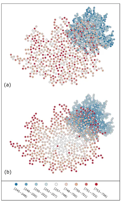
The generated synthetic point locations are assigned normal attribute values from two different populations, which are randomly assigned for spatially uncorrelated cases (Figure 1a). In contrast, the values are ordered ascendingly first, before they are allocated to the points in a radial manner when patterns are spatially structured (Figure 1b). In the interior there are lower values, which increase towards the edges of the respective sub-pattern. The outline of the actual means and standard deviations used is found in Section 2.3.
2.2 Moran’s I
The estimator studied, Moran‟s I, is a measure of spatial autocorrelation. It measures the degree of correspondence between structures in geographic space and those found in an attribute. It reads as (Cliff & Ord 1981, Getis 2010)
∑
∑ ∑ ( ̅)( ̅)
∑ ( ̅)
(1)
where represent attribute values with mean ̅ indexed over spatial units * +. The denote pairwise
positive spatial weights. Moran‟s I is the most frequently used estimator of spatial autocorrelation. It is typically preferred over alternative measures like Geary‟s c for its superior power
characteristics and because it is less prone to statistical and configurational outliers (Chun & Griffith 2013). The applied spatial weights have a distance cut-off at 80 distance units (the upper bound of the large-scale interaction) and follow an inverse distance weighting scheme given by
{| |
| |
(2)
[image:3.595.323.519.293.618.2]This scheme is chosen for resembling the distance-based rules that are used for constructing the patterns (see Section 2.1).
Figure 1. Illustration of the investigated overlapping patterns for μ1 = 250, μ2 = 750, σ1 = σ2 = 1. (a) Spatially random
patterns, (b) spatially autocorrelated patterns.
2.3 Heat maps of I with differing configurations
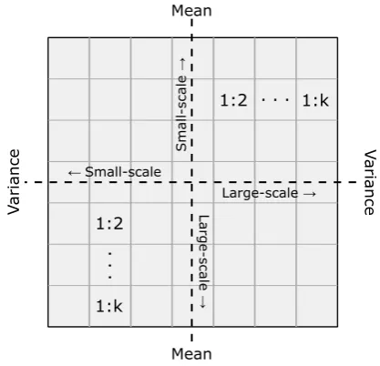
centred, meaning that the mean and variance for both processes are the same (1:1) in the central grid cell. A ratio of, for instance, 1:3 in the left x-direction then means that the mean value of the small-scale pattern is 3 times that of the large-scale pattern. This scheme is illustrated in Figure 2.
Figure 2. Illustration of the applied heat maps. Variable k
denotes the maximum number of multiples of the statistical parameters from the respective other investigated pattern.
3
Results
For all results obtained, the initial means and variances start at μ = 25 and σ² = 400. Depending on which side the heat map is viewed, integer multiples of these values are adapted either for the small-scale (left and up) or for the large-scale sub-pattern (right and down). The multiplication factor thereby corresponds to the number of shifted grid cells. The respective other sub-pattern remains in its initial state and Moran's I is then calculated from the overall pattern in a joint manner, i.e., including both statistically differing populations simultaneously.
3.1 Superposed spatially uncorrelated patterns
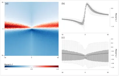
The results for the case of spatially uncorrelated overlapping patterns are given in Figure 3. The Moran‟s I values in the heat map in Figure 3a appear noisy. This is caused by the randomness introduced by the lack of spatial structure in the two overlapping patterns.
The means involved need to be almost identical in order to observe Moran‟s I values close to its expected value of
, - . This is supported by the box plots given in Figure 3b showing that, as soon as one of the involved means is more than three times that of the other, the spatial pattern in the data appears excessively negatively autocorrelated. Further, high positive outliers indicating clustering are only
found on the same interval where the means are nearly identical. These outliers are caused by similar values from the different patterns, which are arbitrarily arranged next to each other by the spatial randomness in the attributes. However, this cannot happen when the means become too different, because all values are then too far away from the overall joint mean value, prohibiting the estimation of positive autocorrelation from the superimposed pattern.
Mean ratios determine the magnitude of Moran‟s I. When the means of the two sub-patterns are very different, the overall spatial autocorrelation tends to be underestimated. The degree of underestimation converges to an almost constant level after the ratio of the means exceeds a factor of 10. Beyond this mark, further differences in the means have only a minor impact on the magnitude of Moran‟s I. The box plots in Figure 3b reveal this effect by the absence of a common trend line. The mean-induced effects are symmetric indicating that it does not matter whether the mean of the small-scale process exceeds the large-scale mean or vice versa.
The ratio of the attribute variances dominates the variability and the range of Moran‟s I. Figure 3c shows that the variability in the estimated I values is small when the variances are roughly identical. In contrast, the dispersion of Moran's I increases when the variances of the two populations become more different. Moran's I then shows a wider range of values with more outliers, both positive and negative. These effects are again symmetric, showing that the scales of the overlapping patterns are not crucially important for a characterisation of spatial autocorrelation when random attribute patterns overlap.
3.2 Superposed spatially autocorrelated patterns
The heat map shown in Figure 4 provides the Moran‟s I
values for the case of spatially structured superimposed patterns. The spatial structuring causes a smoother transition of Moran‟s I over the grid cells of the heat map, meaning that the estimation of the statistic is more predictable with respect to statistical parameters than with superimposed spatially random attributes.
Differences in mean values determine the magnitude of Moran‟s I. In contrast to the symmetric behaviour observed with spatially random patterns, larger means in the small-scale process lead to higher Moran‟s I estimates than vice versa (Figure 4b). The reason is that, because of the applied weighting scheme, more values above the global combined mean value are being related with a relatively high weight, in turn leading to higher I values. This demonstrates a strong interaction between the type of applied spatial weights and the involved superimposed geometric scales.
AGILE 2018 – Lund, June 12-15, 2018
Figure 3: Moran‟s I with superimposed spatially random patterns. (a) Heat map of Moran‟s I values with different mean-variance combinations in the attributes; (b) Box plots summarizing the influences of mean differences (i.e., the
rows); (c) Box plots summarizing the influences of differing variances (i.e., the columns).
Figure 4: Moran‟s I with superimposed spatially autocorrelated patterns. (a) Heat map of Moran‟s I values with different mean-variance combinations in the attributes; (b) Box plots summarizing the influences of mean differences
[image:5.595.84.494.492.753.2]Differing variances play a minor role in comparison to the effects induced by mean differences. One notable observation is made in the case of dominant small-scale variances when the means of the sub-patterns are held almost identical at the same time. A large number of more pronounced positive autocorrelations is found on this interval, and that is caused by the generally larger number of points in the outer parts of the patterns. These feature higher attribute values than the interior parts. When the variance increases, the differences between interiors and outer parts become more pronounced, meaning that more and higher attribute values from one sub-pattern interact with similar ones from the other. This effect vanishes once the small-scale means exceed those of the large-scale pattern by a factor of approximately 15. Further, when the radial attribute pattern is reversed, the same effect appears in reversed form (i.e., the red grid cells in the heat map are then mirrored on the X-axis).
Another variance effect is that the range of Moran‟s I is smallest when the variances of the involved attributes are almost identical. The affected interval is narrow, and there is a sharp but symmetric increase in both magnitude and range of Moran‟s I as soon as either of the variances dominates.
4
Discussion and conclusions
This paper examines the effects of different spatially superimposed statistical populations as those likely to be found in geosocial media data. The results are obtained on a synthetic spatial layout that mimics a partial geometric overlap of different phenomena. The following key insights are obtained:
Different simultaneously present means determine the intensity of Moran‟s I.
Different simultaneously present variances determine the range and variability of Moran‟s I.
Different sub-pattern mean values introduce negative autocorrelation, and thus lead to an underestimation of spatial autocorrelation.
Differences in the means and variances are only marginally influenced by their associated scales when the overlapping patterns are themselves spatially random.
When superimposed patterns are spatially structured, the scale of the pattern associated with the dominant mean value exerts stronger influence on changes in the interpretation of Moran‟s I.
Limitations exist in both the chosen layout as well as the applied spatial weighting scheme. Other geometric forms and interaction types exist, as well as further relevant weighting schemes that are not investigated in this paper. Further, the drawn variates are taken from normal distributions only. Count data or rates are beyond the scope of this paper and deserve treatment in future research. This is especially the case when the overlapping attributes form mixtures not non-symmetric random variables (cf. Griffith 2010).
Despite its relation to spatial analysis, the research carried out in this paper contributes to the recent efforts to develop a GIScience theory of platial analysis. The focus on spatial superposition is thereby interesting, because, other than in traditional GIS, places are spatially overlapping and co-located places must not be mutually related (Goodchild 2015).
This work further supports efforts in other related disciplines facing similar technical issues. The event-sampling method (ESM) from psychology, which collects survey responses in situ, is one such example (Bluemke et al. 2017) for which the obtained results are useful with respect to the design of appropriate analytical approaches and to the interpretation of the collected survey responses.
Future research should consider other geometric setups combined with other types of attributes and dispersal mechanisms. Further, related measures like Geary‟s c or Gi*
might lead to slightly different results, as these combine statistical information in different ways. For instance, unlike Moran‟s I, Geary‟s c estimates covariance through calculating
squared attribute differences, which could change the results obtained in this paper.
Acknowledgments
This work was generously supported by the German Research Foundation (DFG) through the priority programme „Volunteered Geographic Information: Interpretation, Visualisation and Social Computing‟ (SPP 1894).
References
Aldstadt, J. (2010). Spatial clustering. In: Fischer, M. and Getis, A. (eds.) Handbook of Applied Spatial Analysis, Heidelberg, Springer, pp. .279-300.
Assuncao, R.-M. and Reis, E.-A. (1999). A new proposal to adjust Moran's I for population density. Statistics in Medicine, 18(16), 2147-2162.
Bluemke, M., Resch, B., Lechner, C., Westerholt, R. and Kolb, J.-P. (2017). Integrating Geographic Information into Survey Research: Current Applications, Challenges and Future Avenues. Survey Research Methods, 11(3), 307-327.
Chun, Y and Griffith, D.-A. (2013). Spatial Statistics and Geostatistics. London, SAGE.
Cliff, A.-D. and Ord, J.-K. (1981). Spatial Processes. London, Pion.
Getis, A. (2008). A history of the concept of spatial autocorrelation: A geographer's perspective. Geographical Analysis,40(3), 297-309.
Goodchild, M.-F. (2007). Citizens as sensors: the world of volunteered geography. GeoJournal, 69(4), 211-221.
Goodchild, M.-F. (2015). Space, place and health. Annals of GIS, 21(2), 97-100.
AGILE 2018 – Lund, June 12-15, 2018
Lovelace, R., Birkin, M., Cross, P. and Clarke, M. (2016). From big noise to big data: Toward the verification of large data sets for understanding regional retail flows.
Geographical Analysis, 48(1), 59-81.
Oden, N. (1995). Adjusting Moran's I for population density.
Statistics in Medicine, 14(1), 17-26.
Sugovic, M. and Witt, J.-K. (2013). An older view on distance perception: Older adults perceive walkable extents as farther.
Experimental Brain Research, 226(3), 383-391.
Tiefelsdorf, M. and Boots, B. (1997). A note on the extremities of local Moran's Iis and their impact on global
Moran's I. Geographical Analysis, 29(3), 248-257.
Tiefelsdorf, M., Griffith, D.-A. and Boots, B. (1999). A variance-stabilizing coding scheme for spatial link matrices.
Environment and Planning A, 31(1), 165-180.
Waldhör, T. (1996). The spatial autocorrelation coefficient Moran's I under heteroscedasticity. Statistics in Medicine, 15(7‐ 9), 887-892.
Walter, S.-D. (1992). The analysis of regional patterns in health data: II. The power to detect environmental effects.
American Journal of Epidemiology, 136(6), 742-759.
Weiss, E.-M., Kemmler, G., Deisenhammer, E.-A., Fleischhacker, W.-W. and Delazer, M. (2003). Sex differences in cognitive functions. Personality and Individual Differences, 35(4), 863-875.
Wender K.F., Haun D., Rasch B. and Bluemke M. (2003) Context Effects in Memory for Routes. In: Freksa C., Brauer W., Habel C. and Wender K.-F. (eds.) Spatial Cognition III. Lecture Notes in Computer Science (Lecture Notes in Artificial Intelligence), vol. 2685, Heidelberg, Springer, pp. 209-231.
Westerholt, R., Resch, B., and Zipf, A. (2015). A local scale-sensitive indicator of spatial autocorrelation for assessing high-and low-value clusters in multiscale datasets.
International Journal of Geographical Information Science, 29(5), 868-887.
Westerholt, R., Steiger, E., Resch, B., and Zipf, A. (2016). Abundant topological outliers in social media data and their effect on spatial analysis. PLOS ONE, 11(9), e0162360.