Consumption changes, not income changes, predict changes in subjective well being

(1)

warwick.ac.uk/lib-publications Manuscript version: Author’s Accepted Manuscript

The version presented in WRAP is the author’s accepted manuscript and may differ from the published version or Version of Record.

Persistent WRAP URL:

http://wrap.warwick.ac.uk/116283

How to cite:

Please refer to published version for the most recent bibliographic citation information. If a published version is known of, the repository item page linked to above, will contain details on accessing it.

Copyright and reuse:

The Warwick Research Archive Portal (WRAP) makes this work by researchers of the University of Warwick available open access under the following conditions.

practicable the material made available in WRAP has been checked for eligibility before being made available.

Copies of full items can be used for personal research or study, educational, or not-for-profit purposes without prior permission or charge. Provided that the authors, title and full

bibliographic details are credited, a hyperlink and/or URL is given for the original metadata page and the content is not changed in any way.

Publisher’s statement:

Please refer to the repository item page, publisher’s statement section, for further information.

(2)

Manuscript version: Author’s Accepted Manuscript

The version presented in WRAP is the author’s accepted manuscript and may differ from the published version or Version of Record.

(3)

Gordon D. A. Browna _{John Gathergood}b

a_{Department of Psychology, University of Warwick, Coventry, CV4 7AL, United Kingdom.}

Email: [email protected]

b_{School of Economics, University of Nottingham, Nottingham, NG7 2RD, United Kingdom.}

Email: [email protected]

Corresponding author: Gordon D. A. Brown, Department of Psychology, University of

Warwick, COVENTRY, CV4 7AL, United Kingdom.

Email: [email protected]. Tel: +44 7818 423560

Acknowledgements: This study was supported by the Economic and Social Research Council

(U.K.) [grant numbers ES/K002201/1 and ES/P008976/1], the Leverhulme Trust [grant

number RP2012-V-022] and the European Research Council (ERC) under the European

Union’s Horizon 2020 research and innovation programme (grant agreement No 788826).

(4)

Abstract

Does happiness depend on what one earns or what one spends? Income is typically found to

have small beneficial effects on being. However, economic theory suggests that

well-being is conferred not by income but by consumption (i.e., spending on goods and services),

and a person’s level of consumption may differ greatly from their level of income due to saving

behavior and taxation. Moreover, research within consumer psychology has established

relationships between people’s spending in specific categories and their well-being. Here we

show for the first time using panel data that changes in life satisfaction are associated with

changes in consumption, not changes in income. We also find some evidence that increased

conspicuous consumption is more strongly associated with improved well-being than is

increased non-conspicuous consumption.

(5)

Consumption Changes, Not Income Changes, Predict Changes in Subjective Well-being

To what extent, and under what circumstances, are consumers happier when they have

more money? Much research into the relationship between economic circumstances and

subjective well-being has focused on the relationship between income and life satisfaction.

This strand of research has typically relied on the availability of large datasets to underpin the

relevant econometric analyses. It is usually found that income has a small beneficial effect on

the life satisfaction of people within a country at a given time, although effects of changing

GDP within countries over time are smaller or absent and effects of income on affective

well-being are sometimes smaller than effects on more cognitive/evaluative measures (Diener &

Seligman, 2004; Kahneman & Deaton, 2010; Stevenson & Wolfers, 2013).

While a strength of many of these studies is their use of large (and sometimes panel)

datasets, a major limitation is their focus on income rather than (or as well as) consumption.

The distinction matters both because of the difference between income and consumption and

in the light of a large body of work in consumer psychology concerning the effects of different

categories of consumption on well-being. Consumption is correlated with income, but at any

given point in time a person’s consumption level may differ greatly from their income level

due to saving behavior and taxation (Attanasio & Pistaferri, 2016; Meghir & Pistaferri, 2011).

Income may under-predict consumption (e.g., for poor households that receive food stamps, or

for households that borrow money to spend) or over-predict consumption (e.g., for wealthier

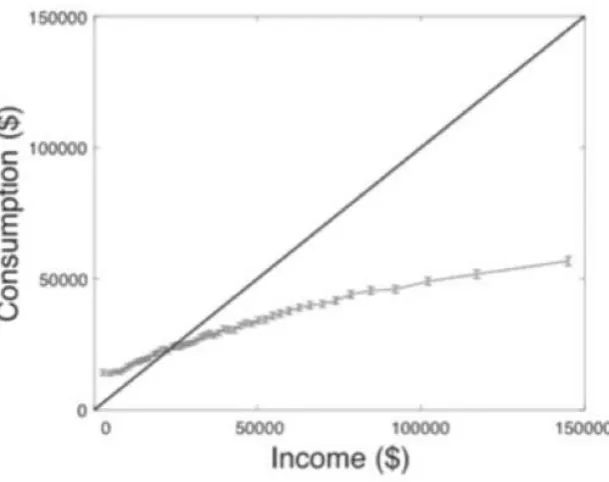
households, which typically save more). In Figure 1 we show that income and consumption

differ substantially among the sample of US households that we describe below. This

difference confirms that current income alone is a poor proxy for consumption of goods and

services. In this paper we therefore ask whether well-being is predicted by consumption,

(6)

[image:6.595.122.427.113.354.2]

Figure 1. Relation between income and consumption. Data are from the Panel Study of Income

Dynamics; see Supplementary Material available online for details. Income data sorted into 50

equally sized bins; points represent mean income and mean consumption within each bin. Error

bars show 95% confidence intervals.

The focus on income, rather than consumption, in econometric analyses of panel data

reflects the lack of available datasets. The few previous large dataset studies of consumption

and general well-being (DeLeire & Kalil, 2010; Headey, Muffels, & Wooden, 2008; Hudders

& Pandelaere, 2012; Noll & Weick, 2015) have mostly been cross-sectional and hence unable

(7)

individual differences (e.g., in personality)1. Moreover, previous studies have typically had

only partial consumption data available. Here in contrast we make use of a large dataset, the

Panel Study of Income Dynamics (PSID) which has complete consumption data (broken down

into categories) for individuals who are tested repeatedly. We exploit the panel structure of the

data to compare the effects of income changes and consumption changes as predictors of

changes in people’s life satisfaction.

Income might plausibly influence well-being even when conventional categories of

consumption are accounted for, perhaps because of savings or feelings of future security.

However the need to focus on the effects of consumption as well as of income on well-being

is confirmed by research (from both economics and psychology) that has focused on different

subcategories of consumption. Research in consumer psychology has typically focused on the

distinction between experiential and material consumption, research in social psychology has

examined effects of prosocial spending, and economic studies have placed more emphasis on

differential effects of conspicuous and non-conspicuous consumption.

Thus one suggestion is that only expenditure on experiential, rather than material, goods

leads to increased well-being (Gilovich & Kumar, 2015; Guevarra & Howell, 2015; Van Boven

& Gilovich, 2003) (although see Schmitt, Brakus, & Zarantonello, 2015). Thinking about past

experiential purchases improves mood more than does thinking about past material purchases,

experiences enter more strongly than do material items into people’s self-narratives (Carter &

Gilovich, 2012), and people are relatively more willing to wait for experiences than for

possessions (Kumar & Gilovich, 2016). Most of this research is laboratory-based and examines

1_{Headey et al. (2008) report a fixed effects analysis of satisfaction with standard of}

living, using partial consumption data and finding a positive effect of consumption in British

(8)

the changes in affect associated with particular expenditures rather than the effect of general

consumption levels on a more cognitive/reflective measure of overall satisfaction with life,

although DeLeire and Kalil (2010) found, in analysis of a large dataset, that amongst older

Americans only leisure consumption was substantially and significantly related to life

satisfaction. DeLeire and Kalil also find a small positive effect of spending on charity and gifts.

Consistent with the latter finding, a third line of research has found positive effects of prosocial

spending on well-being (e.g., Dunn, Aknin, & Norton, 2008; Goodman, Lim, & Meyvis, 2017;

Whillans, Dunn, Sandstrom, Dickerson, & Madden, 2016).

Research within economics has in contrast emphasized the role of conspicuous or

positional consumption in conferring status-related utility (Frank, 2010; Saad, 2011; Veblen,

1899), consistent with a large body of research suggesting that the desire for status is a basic

human concern (Anderson, Hildreth, & Howland, 2015). Some correlational evidence is

consistent with a link between well-being and conspicuous consumption (Hudders &

Pandelaere, 2012, 2015; Masferrer-Dodas, Rico-Garcia, Huanca, Reyes-Garcia, & Team,

2012). While the literature on income and positional consumption differs from much research

in consumer psychology in the well-being measures that are typically used (i.e., often using

measures of cognitive/reflective rather than affective well-being), as well as in the manner in

which overall consumption is subdivided, it is possible that “experiential consumption” and

“conspicuous consumption” are at least partially overlapping categories. We return to this issue

below.

Here we address these issues in a novel way by making use of the PSID. This brings

two key advantages. First, use of panel data (in which the same individuals are surveyed on

more than one occasion) enables us to examine whether within-individual changes in economic

circumstances (whether of income or consumption) are associated with within-individual

(9)

achievable using cross-sectional data alone. Most previous results have not only been confined

to the study of income rather than consumption, but also have been cross-sectional (for

exceptions, see e.g. Cheng, Powdthavee, & Oswald, 2015; Hounkpatin, Wood, Brown, &

Dunn, 2015). Second, complete consumption data are available for individuals, broken down

by categories. This not only enables a more global examination of the effects of consumption

on well-being than is typical in the consumer psychology literature (in our dataset only about

5% of consumption expenditure is on vacations and hobbies, which are the categories closest

to “experiential” consumption), but allows us to look at sub-categories of consumption. We

first ask whether it is income, or consumption, that affect overall satisfaction with life. Income

can, after all, be allocated to material, experiential, or prosocial spending at the recipient’s

discretion. Taking an exploratory approach, we then look at possible differential effects of

different categories of consumption on well-being with a particular focus on the distinction

between conspicuous and non-conspicuous consumption.

Throughout, we focus on “fixed effects” analyses which exploit the panel structure of

the data and focus on within-individual changes in the variables of interest.2 While the results

from conventional cross-sectional regression analyses allow comparison of the effects of

consumption (and its subcategories) with the effects of income across individuals, such

analyses are limited in that they are susceptible to third-variable problems – there might be

some unmeasured individual characteristic (such as personality) which is correlated with both

well-being and spending behavior. The fixed effects analyses examine whether

within-individual changes over time in one variable (e.g., consumption) can predict within-within-individual

2_{The term “fixed effects” is used in a number of different ways in different literatures}

(see, e.g., Gelman, 2005). Our usage is most common in econometrics, and refers to estimating

(10)

changes in the outcome variable (well-being) after controlling for changes in other predictors.

The analyses therefore effectively control for the effects of unobservable but relatively stable

individual differences (e.g., in personality, although see Boyce, Wood, & Powdthavee, 2013;

Luhmann, Orth, Specht, Kandler, & Lucas, 2014) that might otherwise represent confounds.

Although the results from fixed effects analyses cannot exclude the possibility that some

causally relevant unobserved variable is changing over time within individuals, and are

informative solely about within-individuals effects, the fixed effects analyses represent a more

conservative approach than conventional cross-sectional regression. At the same time, these

analyses address different theoretical questions to those addressed by cross-sectional analyses,

and the fixed effects results that we report below cannot support claims about

between-individual relationships.

Analysis 1: Does income or consumption affect well-being?

Our first analysis examines whether income or consumption influences subjective

well-being. The PSID provides detailed consumption data on household expenditures in 34

categories as well as a measure of well-being and various control variables (Andreski, Li,

Samancioglu, & Schoeni, 2014).

Method

Our use of the PSID is motivated by the fact that, our knowledge, it is the only large scale

household panel survey that includes both measures of life satisfaction and detailed

consumption data. Full details of participants, data collection methods, and measures used in

the survey are available at psidonline.isr.umich.edu/Guide/documents.aspx. We use the three

most recently available waves — 2009, 2011 and 2013 — which include information on life

(11)

PSID has included a standard self-reported life satisfaction question phrased as follows:

‘Please think about your life as a whole. How satisfied are you with it? Are you completely

satisfied, very satisfied, somewhat satisfied, not very satisfied, or not at all satisfied?’ This

question is asked only of the main respondent, who also answers the household questionnaire.

Consequently, we use data on only one respondent per household. Our sample is therefore not

fully representative of the US adult population as it under-represents second and third adult

members of household units (typically spouses), with 74% of the respondents in our sample

being male. We restrict the sample to a balanced panel of households. We decided ahead of

time to omit observations which fall into the top 1% or bottom 1% of the distribution of

consumption or income, as there are typically extreme outliers (e.g., one or two incomes in the

millions of dollars, or reports of negative income and/or consumption) and hence such omission

is standard practice in econometric analyses.3

This left us with 16,992 observations for 5,664 individuals. Sample size was therefore

determined entirely by the nature of the sample available to us along with the above-mentioned

exclusionary criteria; no stopping rule was applied in our analyses. The STATA scripts used to

conduct the analyses are available in the online Supplementary Material. We have reported the

results of all analyses that were undertaken,

Summary data for demographics, socio-economic controls and the measure of life

satisfaction for the three waves of data pooled together are shown in the Supplementary

Material available online (Table S1). Among the balanced panel of individual-year

observations 74% are for male individuals, with an average age of 46. Approximately half of

the sample are married or have a partner, two-thirds have high school education or higher, more

3_{We nonetheless repeated all analyses without the exclusions at the request of a referee}

(12)

than two-thirds are employed and a little over 60% own their home. Average self-reported

health is 3.5 (mid-way between ‘good’ and ‘very good’), and the mean score on the Kessler

mental anxiety scale is 3.8 out of a possible 24. The average value of life satisfaction is 3.8,

with a standard deviation of 0.83. Equivalized total consumption (i.e. consumption per

household member) and consumption by main PSID category are summarized in Table S2 in

the Supplementary Material. The PSID consumption data are consistent with more detailed

consumption data in the Consumer Expenditure Survey. The table reports the unconditional

means and standard deviation (i.e. including zero values), hence the individual row means sum

to the mean of total consumption. The largest single consumption category is housing (36% of

total expenditure), followed by transport (19%) and food (15%). Summary data for the

sub-categories which together comprise these main sub-categories are shown in the online

Supplementary Material (Tables S3 and S4).

Results

Our main analysis estimates the following equation:

𝐿𝑆_{𝑖,𝑠,𝑡} = 𝛽₁log⁡(𝐶)_{𝑖,𝑠,𝑡}+ 𝛽₂log⁡(𝑌)_{𝑖,𝑠,𝑡}+ 𝛽₃X_{𝑖,𝑠,𝑡} + 𝜃_𝑖 + 𝜇_𝑠 + 𝜑_𝑡+ 𝜖_{𝑖,𝑠,𝑡}⁡⁡⁡⁡⁡⁡⁡(1)

where individual i lives in state s in time period, t, log(C) is the natural log of total equivalized

annual consumption, log(Y) is the natural log of equivalized annual income, X is a vector of

time-varying demographic and socio-economic controls and 𝜃, 𝜇, and 𝜑⁡are individual, state

and time fixed effects. The time dimension of our data covers three waves: 2009, 2011 and

2013. In our baseline specification, consumption and income enter as their natural logs. To

ensure robustness, we also estimate models in which consumption and income enter in levels

(13)

As the majority of our analyses used the fixed effects method, in the Supplementary

Material we report overall between-subjects and within-subjects standard deviations for our

main variables (consumption and income: Table S5), main consumption categories (Table S6),

and socio-economic covariates (Table S7).

Our main econometric model regresses life-satisfaction (on a 5-point scale) against the

natural log of equivalized household consumption; the natural log of equivalized household

income; individual, geographic state of residence and time fixed effects, and controls. The key

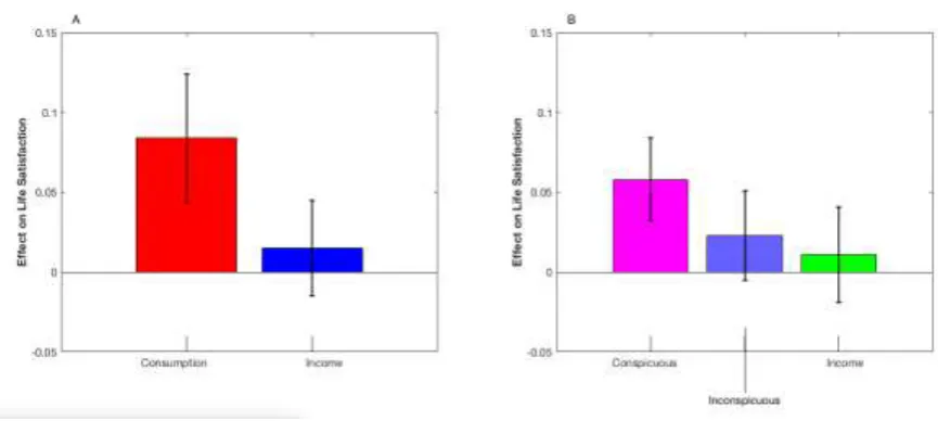
coefficients are shown in Figure 2A, with full results in Table 1.

[image:13.595.118.551.379.573.2]

Figure 2. Coefficients predicting life satisfaction from income and consumption. Data are from

the Panel Study of Income Dynamics. A: Coefficients on log(overall consumption) and

log(income). B: Coefficients on log(conspicuous consumption), log(inconspicuous

consumption) and log(income). All coefficients are from regressions that include controls.

(14)

In Columns 1 and 2 of Table 1 we show univariate models (i.e. without any controls or

fixed effects) in which life satisfaction is regressed against log income (Column 1) and log

consumption (Column 2) for the most recent (2013) wave of data.4 The variance inflation

factors were 1.03 (life satisfaction), 1.88 (log consumption), and 1.89 (log income), indicating

acceptable levels of collinearity. We then turn to the main analyses and include individual fixed

effects in Columns 3 and 4,

(15)

Table 1: Main regression estimates, log specification. Table reports regression estimates [95% Cis] for the balanced PSID panel 2009-2013.

Columns 1 and 2 are pooled cross-section regressions for the year 2013; Columns 3 - 7 include individual fixed effects. Education refers to highest

educational qualification obtained by the respondent. Employment refers to current employment status. Self-reported health question in full is:

`Would you say your health in general is excellent, very good, good, fair, or poor?' We code excellent = 5, poor = 1. Mental Anxiety Scale is

derived from responses to the Kessler-6 non-specific psychological distress scale.

(1) (2) (3) (4) (5) (6) (7)

Pooled Pooled Fixed Effects Fixed Effects Fixed Effects Fixed Effects Fixed Effects

Log Consumption 0.219 0.103 0.098 0.083 0.084

[0.179,0.259] [0.065,0.140] [0.059,0.137] [0.043,0.122] [0.045,0.124]

Log Income 0.179 0.033 0.018 0.009 0.015

[0.152,0.205] [0.004,0.062] [-0.012,0.047] [-0.021,0.039] [-0.015,0.045]

Age 0.027 -0.029

[-0.026,0.080] [-0.097,0.040]

Age Squared -0.000 0.000

[-0.001,0.001] [-0.001,0.001]

Age Cubed 0.000 -0.000

[-0.000,0.000] [-0.000,0.000]

Married / Partner (= 1) 0.103 0.094

[-0.012,0.218] [-0.021,0.209]

Widowed (= 1) 0.105 0.071

[-0.142,0.352] [-0.177,0.319]

Divorced (= 1) 0.015 -0.004

[-0.133,0.163] [-0.152,0.145]

Separated (= 1) -0.230 -0.239

[-0.385,-0.076] [-0.393,-0.085]

[image:15.842.79.764.219.526.2]

(16)

[0.011,0.063] [0.015,0.067]

Highschool Graduate (= 1) 0.109 0.096

[0.001,0.217] [-0.012,0.205]

College graduate (= 1) 0.048 0.059

[-0.078,0.174] [-0.068,0.185]

GED (= 1) 0.050 0.036

[-0.177,0.276] [-0.190,0.263]

Employed (= 1) 0.006 0.003

[-0.047,0.059] [-0.050,0.056]

Unemployed (= 1) -0.154 -0.158

[-0.221,-0.088] [-0.224,-0.092]

Temp. Non-Working (= 1) -0.036 -0.035

[-0.201,0.130] [-0.201,0.131]

Owns Home (=1) 0.046 0.041

[-0.038,0.130] [-0.043,0.126]

Rents Home (=1) 0.036 0.033

[-0.039,0.112] [-0.043,0.108]

Self-Reported Health (1-5) 0.090 0.089

[0.072,0.108] [0.070,0.107]

Mental Anxiety Scale -0.017 -0.021

[-0.021,-0.013] [-0.025,-0.017]

Observations 16992 16992 16992 16992 16992 16992 16992

State Fixed Effects No No No No No No Yes

(17)

CONSPICUOUS CONSUMPTION AND WELL-BEING

16

where it is evident that the magnitude of the coefficient on log consumption reduces by a half

and the coefficient on log income reduces to only one fifth of its previous magnitude. These

results confirm that controlling for individual level heterogeneity is very important in life

satisfaction estimates. When we include both log consumption and log income together

(Column 5) we find that the coefficient on log consumption is estimated to be greater than zero,

whereas the coefficient on log income is not. A t-test of equivalence confirms that the

coefficients are statistically significantly different from one another (p =.0030). The coefficient

on log consumption is five times larger than the coefficient on log income. With the addition

of socio-economic and demographic controls (Column 6) the coefficient on log consumption

falls slightly in magnitude but it increases very slightly when we add state of residence and

year fixed effects (Column 7).

Thus, there is a positive effect of consumption upon life satisfaction (β = 0.084, 95%

CI [0.045, 0.124]), but no evidence for an effect of income, in the most conservative analysis

(Column 7). The coefficient estimates imply that the effect of an increase in consumption is at

least five times as large as the effect of the same increase in income, when they are treated as

independent: A one standard deviation increase in consumption leads to an increase in life

satisfaction of approximately 5.2% of a standard deviation. We find very similar effects when

estimating models in which income and consumption enter in levels, not log (see Table S8 in

Supplementary Material for results).

Discussion

Our results show that consumption changes, not income changes, predict changes in

life satisfaction. We note possible implications for public policy. There has been much recent

(18)

17

evaluated, at least in part, in terms of their effects on population well-being (Dolan &

Kahneman, 2008; O’Donnell, Deaton, Durand, Halpern, & Layard, 2014). While previous

studies use income-equivalents of well-being effects, our analysis suggests that the increases

in consumption that would be required to compensate for the negative effect of specific life

events on life satisfaction (consumption–equivalents) would differ.

Analysis 2: Effects of Different Categories of Consumption

The detailed consumption data available for this study allow us to examine the

relationship between different types of consumption and life satisfaction, and we do this in

Analysis 2. To our knowledge, ours is the first study to do so using detailed consumption

microdata in a panel survey design.

In analyzing the effects of subcategories of consumption, we adopt a conservative

approach. We first present results in a theory-neutral way by examining the effects of each

major subcategory of consumption on well-being after controlling for income and other

background variables. These analyses therefore make no assumption about the “correct” way

to group consumption categories together, and we include all the code for analysis so that other

researchers may construct their own groupings. However, given that there already exists a large

prior literature suggesting that conspicuous consumption is an important category, we then take

advantage of an independently-motivated categorization of consumption types as

“conspicuous” and “non-conspicuous” to examine the differential relations of these

subcategories of consumption to well-being.

Method

Table 2 shows the intercorrelation matrix between life satisfaction, income, total

(19)

18

Table 2: Correlations between life satisfaction, income, total consumption, and all major

categories of consumption as defined in the PSID.

Life Satisfaction

Income Total

Cons

Food Housing Utilities Transport School Childcare Healthcare Home

Repairs

Home Furnishings

Clothing Holidays Hobbies

Life Satisfaction 1

Income 0.151 1

Total Consumption 0.123 0.645 1

Food 0.0877 0.406 0.552 1

Housing 0.0838 0.558 0.788 0.337 1

Utilities 0.0454 0.172 0.361 0.160 0.366 1

Transport 0.0580 0.300 0.568 0.209 0.209 0.106 1

School 0.0388 0.166 0.321 0.101 0.106 0.0214 0.0672 1

Childcare 0.0424 0.0958 0.133 0.0217 0.0695 -0.0221 0.0268 0.00997 1

Healthcare 0.0546 0.276 0.402 0.203 0.180 0.119 0.140 0.0669 0.0209 1

Home Repairs 0.0544 0.212 0.435 0.126 0.361 0.129 0.0736 0.0367 0.0225 0.125 1

Home Furnishings 0.0395 0.199 0.358 0.151 0.286 0.0595 0.0936 0.0247 0.0338 0.0721 0.154 1

Clothing 0.0277 0.219 0.329 0.191 0.180 0.0409 0.106 0.0655 0.0455 0.0499 0.0740 0.209 1

Holidays 0.117 0.397 0.439 0.261 0.261 0.0841 0.129 0.0901 0.0145 0.156 0.145 0.150 0.236 1

Hobbies 0.0398 0.257 0.313 0.199 0.172 0.00672 0.0971 0.0588 0.0150 0.0975 0.0805 0.112 0.222 0.233 1

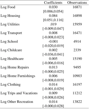
We first report the coefficients relating each PSID category of consumption to life satisfaction,

using the fixed effects specification and all the controls (income and socio-demographic

variables) used in the analyses reported above. Our aim here is to present an exploratory and

“theory neutral” analysis prior to exploiting an independently-developed classification of

consumption categories as “conspicuous” or “non-conspicuous”. The results can be seen in

Table 3, where it is evident that there are effects of spending in a number of different

[image:19.595.48.575.175.411.2]

(20)

[image:20.595.157.446.160.513.2]

19

Table 3. Coefficients relating each PSID category of consumption to life satisfaction,

using the fixed effects specification and all controls.

Coefficients Observations

Log Food 0.030 16871

[0.006,0.054]

Log Housing 0.084 16898

[0.051,0.116]

Log Utilities .019 15959

[-0.009,0.047]

Log Transport 0.008 16471

[-0.008,0.023]

Log School -0.001 4914

[-0.020,0.019]

Log Childcare 0.002 2339

[-0.036,0.041]

Log Healthcare 0.005 15190

[-0.006,0.016]

Log Home Repairs 0.013 9495

[-0.000,0.025]

Log Home Furnishings 0.006 10903

[-0.008,0.019]

Log Clothing 0.014 16197

[-0.001,0.029]

Log Trips and Vacations 0.009 11212

[-0.008,0.026]

Log Other Recreation 0.014 13822

[-0.000,0.028]

For a more theory-driven analysis of conspicuous consumption, we assign each

sub-category as ‘conspicuous’ or ‘non-conspicuous’. We draw on data constructed by Heffetz

(2011) who commissioned a survey of a representative sample of US consumers who were

asked to evaluate the visibility of different consumption types. Respondents to the survey were

asked to evaluate 31 consumption categories with results indicating cigarettes to be most visible

category of expenditure and, perhaps unsurprisingly, underwear to be the least visible category.

The author uses those data to predict how consumption in different categories changes as a

(21)

20

income when the consumption is more visible. This result is consistent with a model in which

consumers gain additional utility from consumption which is conspicuous. In our baseline

classification, we mapped all the PSID expenditure categories to the Heffetz classification, and

classified as “conspicuous” all and only all the PSID categories that appeared in the top half of

the ranking reported by Heffetz (2011). These were: food away from home, clothing, holidays,

recreation / hobbies and expenditure on telephones.

In additional classifications, we examine the sensitivity of results to including home

furnishings and schooling as ‘conspicuous’ (see below, and Supplementary Material).

Depending upon which classification we use, the share of conspicuous consumption among the

PSID sample ranges at the mean between one quarter to one third of total consumption.

Result

Table 4 presents estimates in which the natural log of total conspicuous and

non-conspicuous consumption enter into the econometric specification separately. The striking

result in Column 1 is that, when we include both conspicuous and non-conspicuous

consumption in the same specification, only the coefficient on conspicuous consumption is

estimated to be different from zero, although a t-test of equivalence found that the coefficients

were not statistically significantly different from one another at the conventional level (p =

0.1050). Columns 2 and 3 show that, even when the variables are entered separately, the

coefficient on non-conspicuous consumption is half the magnitude of that on conspicuous

consumption. As a sensitivity test, we also estimate the same model specifications, but with

Table 4: Conspicuous and non-conspicuous consumption, log specification. Table reports

individual fixed effects regression estimates (SEs) for balanced PSID panel 2009 -2013. For

categorization of consumption components into 'conspicuous' and 'non-conspicuous'

consumption groups see main text. Education refers to highest educational qualification

obtained by the respondent. Employment refers to current employment status. Self-reported

(22)

21

fair, or poor?' We code excellent = 5, poor = 1. Mental Anxiety Scale is derived from responses

to the Kessler-6 non-specific psychological distress scale. Control variables not shown:

housing tenure dummies.

(1) (2) (3)

Fixed Effects Fixed Effects Fixed Effects

Log Conspicuous Consump. 0.058 0.061

[0.031,0.084] [0.035,0.087]

Log Non-Conspic. Consump. 0.023 0.033

[-0.005,0.051] [0.005,0.061]

Log Income 0.011 0.014 0.020

[-0.019,0.041] [-0.015,0.044] [-0.010,0.050]

Age -0.026 -0.025 -0.026

[-0.094,0.042] [-0.093,0.044] [-0.094,0.043]

Age Squared -0.000 -0.000 -0.000

[-0.001,0.001] [-0.001,0.001] [-0.001,0.001]

Age Cubed -0.000 -0.000 -0.000

[-0.000,0.000] [-0.000,0.000] [-0.000,0.000]

Married/Partner (= 1) 0.093 0.093 0.092

[-0.022,0.208] [-0.022,0.208] [-0.022,0.207]

Widowed (= 1) 0.065 0.067 0.071

[-0.183,0.313] [-0.181,0.315] [-0.177,0.319]

Divorced (= 1) -0.006 -0.006 -0.005

[-0.154,0.142] [-0.154,0.142] [-0.153,0.144]

Separated (= 1) -0.240 -0.239 -0.238

[-0.394,-0.085] [-0.394,-0.085] [-0.392,-0.084]

No. Dependent Children 0.041 0.040 0.036

[0.015,0.067] [0.014,0.066] [0.010,0.062]

Highschool Graduate (= 1) 0.098 0.099 0.097

[-0.010,0.207] [-0.010,0.207] [-0.012,0.205]

College graduate (= 1) 0.058 0.060 0.060

[-0.068,0.185] [-0.067,0.186] [-0.066,0.187]

GED (= 1) 0.038 0.036 0.033

[-0.188,0.265] [-0.190,0.262] [-0.194,0.259]

Employed (= 1) 0.002 0.003 0.004

[-0.051,0.055] [-0.050,0.056] [-0.049,0.057]

Unemployed (= 1) -0.158 -0.159 -0.159

[-0.224,-0.092] [-0.225,-0.093] [-0.226,-0.093]

Temp. Non-Working (= 1) -0.032 -0.030 -0.033

[-0.198,0.134] [-0.196,0.136] [-0.199,0.133]

Self-Reported Health (1-5) 0.088 0.088 0.089

[0.070,0.107] [0.069,0.106] [0.071,0.107]

(23)

22

[-0.025,-0.017] [-0.025,-0.017] [-0.025,-0.017]

Observations 16992 16992 16992

consumption and income entering in levels (in units of ten thousand dollars), not log values

(see Table S9 in online Supplementary Material for results). The pattern in the coefficient

estimates is very similar to that in Table 4, with the exception that the estimate of the coefficient

of non-conspicuous consumption is not estimated to be different from zero in either

specification in which it enters and a t-test of equivalence confirms that the difference between

the coefficients approached the conventional level of statistical significance (p = 0.051). In

further sensitivity tests we i) excluded the measure of psychological anxiety from the

specification and also ii) excluded the measure of income from the specification. In both cases

results are unchanged.

As a sensitivity test, we change classifications of sub-categories of consumption across

groups. We see very similar results to those in the main tables (see Table S10 in Supplementary

Material for full results). When we include home furnishings in the conspicuous category, the

coefficient on the conspicuous consumption variable falls in magnitude and the coefficient on

the non-conspicuous consumption variable increases in magnitude. The same occurs to a lesser

extent when we also include school expenses in the conspicuous category. In both joint

specifications the coefficient on conspicuous consumption is more precisely estimated and

larger in magnitude than the coefficient on the non-conspicuous consumption variable.

Next, we note that it has recently been argued that the effects of income on well-being

reflect social comparison processes, and that is the relative rank of a person’s income within a

comparison group, rather than income per se, that is positively associated with well-being (e.g.,

(24)

23

same is true for consumption. With the data we use here it is not possible to distinguish between

these possibilities, because the correlations between consumption and consumption rank are

very high. For example, rank of overall consumption is correlated .978 with log overall

consumption, and .938 with overall consumption level. For conspicuous consumption, the

correlations are .964 and .836 respectively. Although it may be possible to separate rank effects

and level effects by making use of different assumed comparison groups, such analyses fall

outside the scope of the present investigation.

Finally, we returned to the issue of whether the relevant categorization of consumption,

for the purposes of predicting life satisfaction, is conspicuous vs. non-conspicuous or

experiential vs. non-experiential. Experiential purchases such as vacations are often social and

highly visible, likely to be mentioned on social media, and the well-being benefit associated

with experiential goods is diminished if people are forbidden from talking about them (Kumar

& Gilovich, 2015). Set against this, it has been suggested that the beneficial effect on

well-being of experiential rather than material consumption reflects the fact that social comparison

is easier for material goods (Howell & Hill, 2009; Van Boven, 2005).

We do not have data on the purchasing intentions of our participants, so any analysis

must be tentative. However two of the sub-categories of consumption in our dataset appear to

be relatively unambiguously classifiable as experiential — expenditure on trips and vacations,

and expenditure on hobbies/recreation. We therefore calculated, for each individual, (a)

consumption falling within these two categories, which we label “experiential”, and (b) all

remaining consumption (“non-experiential”). We then conducted fixed effect analyses

paralleling those reported above for conspicuous and non-conspicuous consumption, and the

results are reported in Tables S11 (log specification) and S12 (level specification) in

(25)

24

coefficients of similar magnitudes for experiential and non-experiential consumption when the

two categories were entered simultaneously and we cannot reject the null hypothesis of

equivalence of coefficients (p = 0.775), although the coefficient on non-experiential

consumption only just failed to reach significance at the conventional level, and both predicted

life satisfaction when entered separately (columns 2 and 3). Table S12 reveals a fairly similar

pattern, although when the two categories are entered simultaneously the difference between

coefficients was marginally significant (p = 0.08). Estimates are evidently sensitive to model

specification, so we consider these results to be inconclusive as to the effects of experiential

and non-experiential consumption on life satisfaction.

General Discussion

Ours is the first study to use large-scale longitudinal household panel microdata with

comprehensive consumption data to address the relationship between consumption and

well-being. Our findings demonstrate the importance of using consumption, as opposed to income,

to estimate the effects of economic resources upon well-being and in the use of such effects to

value non-market goods. Our use of a panel design (fixed-effects specification) goes some way

towards ruling out the possibility that our results reflect time-invariant confounding individual

differences like personality (e.g., individuals high in extraversion might both consume more

and experience higher well-being), although the possible existence of an unknown and causally

relevant third variable cannot be ruled out.

Our study relates to a large existing literature in both economics and psychology. It has

often been suggested that increased spending may actually reduce well-being (Frank, 2004;

Scitovsky, 1976) and, empirically, materialistic attitudes are associated with reduced

well-being on a number of dimensions (Kashdan & Breen, 2007; Kasser, 2002). Our results speak

(26)

25

increased spending but they leave open the possibility that more affect-related aspects of

(27)

26 References

Anderson, C., Hildreth, J. A. D., & Howland, L. (2015). Is the desire for status a fundamental

human motive? A review of the empirical literature. Psychological Bulletin, 141(3),

574-601.

Andreski, P., Li, G., Samancioglu, M. Z., & Schoeni, R. (2014). Estimates of annual

consumption expenditures and its major components in the PSID in comparison to the

CE. American Economic Review, 104(5), 132-135.

Attanasio, O. P., & Pistaferri, L. (2016). Consumption inequality. Journal of Economic

Perspectives, 30(2), 3-28.

Boyce, C. J., Brown, G. D. A., & Moore, S. C. (2010). Money and happiness: Rank of

income, not income, affects life satisfaction. Psychological Science, 21, 471-475.

Boyce, C. J., Wood, A. M., & Powdthavee, N. (2013). Is personality fixed? Personality

changes as much as "variable" economic factors and more strongly predicts changes

to life satisfaction. Social Indicators Research, 111(1), 287-305.

Carter, T. J., & Gilovich, T. (2012). I am what I do, not what I have: The differential

centrality of experiential and material purchases to the self. Journal of Personality

and Social Psychology, 102(6), 1304-1317.

Cheng, T. C., Powdthavee, N., & Oswald, A. J. (2015). Longitudinal evidence for a midlife

nadir in human well-being: Results from four data sets. The Economic Journal.

DeLeire, T., & Kalil, A. (2010). Does consumption buy happiness? Evidence from the United

States. International Review of Economics, 57(2), 163--176.

Diener, E., & Seligman, M. E. P. (2004). Beyond money: Toward an economy of well-being.

Psychological Science in the Public Interest, 5, 1-31.

Dolan, P., & Kahneman, D. (2008). Interpretations of utility and their implications for the

valuation of health. The Economic Journal, 118(525), 215-234.

Dunn, E. W., Aknin, L. B., & Norton, M. I. (2008). Spending money on others promotes

happiness. Science, 319(5870), 1687-1688.

Frank, R. H. (2004). How not to buy happiness. Daedalus, 133(2), 69-79.

Frank, R. H. (2010). Luxury fever: Weighing the cost of excess. Princeton, NJ: Princeton

(28)

27

Gelman, A. (2005). Analysis of variance - Why it is more important than ever. Annals of

Statistics, 33(1), 1-31.

Gilovich, T., & Kumar, A. (2015). We'll Always Have Paris: The Hedonic Payoff from

Experiential and Material Investments. Advances in Experimental Social Psychology,

Vol 51, 51, 147-187.

Goodman, J. K., Lim, S., & Meyvis, T. (2017). When consumers prefer to give material gifts

instead of experiences: The role of social distance. Journal of Consumer Research.

Guevarra, D. A., & Howell, R. T. (2015). To have in order to do: Exploring the effects of

consuming experiential products on well‐being. Journal of Consumer Psychology,

25(1), 28-41.

Headey, B., Muffels, R., & Wooden, M. (2008). Money does not buy happiness: Or does it?

A reassessment based on the combined effects of wealth, income and consumption.

Social Indicators Research, 87(1), 65-82.

Heffetz, O. (2011). A test of conspicuous consumption: Visibility and income elasticities.

Review of Economics and Statistics, 93(4), 1101-1117.

Hounkpatin, H. O., Wood, A. M., Brown, G. D. A., & Dunn, G. (2015). Why does income

relate to depressive symptoms? Testing the income rank hypothesis longitudinally.

Social Indicators Research, 124(2), 637-655.

Howell, R. T., & Hill, G. (2009). The mediators of experiential purchases: Determining the

impact of psychological needs satisfaction and social comparison. The Journal of

Positive Psychology, 4(6), 511-522.

Hudders, L., & Pandelaere, M. (2012). The silver lining of materialism: The impact of luxury

consumption on subjective well-being. Journal of Happiness Studies, 13(3), 411-437.

Hudders, L., & Pandelaere, M. (2015). Is having a taste of luxury a good idea? How use vs.

Ownership of luxury products affects satisfaction with life. Applied Research in

Quality of Life, 10(2), 253-262.

Kahneman, D., & Deaton, A. (2010). High income improves evaluation of life but not

emotional well-being. Proceedings of the National Academy of Sciences of the United

States of America, 107(38), 16489-16493.

Kashdan, T. B., & Breen, W. L. (2007). Materialism and diminished well-being: Experiential

avoidance as a mediating mechanism. Journal of Social and Clinical Psychology,

26(5), 521-539.

(29)

28

Kumar, A., & Gilovich, T. (2015). Some "thing" to talk about? Differential story utility from

experiential and material purchases. Personality and Social Psychology Bulletin,

41(10), 1320-1331.

Kumar, A., & Gilovich, T. (2016). To do or to have, now or later? The preferred consumption

profiles of material and experiential purchases. Journal of Consumer Psychology,

26(2), 169-178.

Luhmann, M., Orth, U., Specht, J., Kandler, C., & Lucas, R. E. (2014). Studying changes in

life circumstances and personality: It's about time. European Journal of Personality,

28(3), 256-266.

Masferrer-Dodas, E., Rico-Garcia, L., Huanca, T., Reyes-Garcia, V., & Team, T. B. S.

(2012). Consumption of market goods and wellbeing in small-scale societies: An

empirical test among the Tsimane' in the Bolivian Amazon. Ecological Economics,

84, 213-220.

Meghir, C., & Pistaferri, L. (2011). Earnings, consumption and life cycle choices. Handbook

of Labor Economics, 4, 773-854.

Noll, H.-H., & Weick, S. (2015). Consumption expenditures and subjective well-being:

empirical evidence from Germany. International Review of Economics, 62(2),

101--119.

O’Donnell, G., Deaton, A., Durand, M., Halpern, D., & Layard, R. (2014). Wellbeing and

policy. Retrieved from London, UK:

Saad, G. (2011). Consuming instinct. New York: Prometheus.

Schmitt, B., Brakus, J. J., & Zarantonello, L. (2015). From experiential psychology to

consumer experience. Journal of Consumer Psychology, 25(1), 166-171.

Scitovsky, T. (1976). The joyless economy: An inquiry into human satisfaction and consumer

dissatisfaction.

Stevenson, B., & Wolfers, J. (2013). Subjective well-being and income: Is there any evidence

of satiation? American Economic Review, 103(3), 598-604.

Van Boven, L. (2005). Experientialism, materialism, and the pursuit of happiness. Review of

General Psychology, 9(2), 132.

Van Boven, L., & Gilovich, T. (2003). To do or to have? That is the question. Journal of

Personality and Social Psychology, 85(6), 1193-1202.

Veblen, T. (1899). The theory of the leisure class. New York: The New American Library.

Whillans, A. V., Dunn, E. W., Sandstrom, G. M., Dickerson, S. S., & Madden, K. M. (2016).

(30)