Effective condition number bounds for convex regularization

warwick.ac.uk/lib-publications

Manuscript version: Author’s Accepted Manuscript

The version presented in WRAP is the author’s accepted manuscript and may differ from the

published version or Version of Record.

Persistent WRAP URL:

http://wrap.warwick.ac.uk/126408

How to cite:

Please refer to published version for the most recent bibliographic citation information.

If a published version is known of, the repository item page linked to above, will contain

details on accessing it.

Copyright and reuse:

The Warwick Research Archive Portal (WRAP) makes this work by researchers of the

University of Warwick available open access under the following conditions.

Copyright © and all moral rights to the version of the paper presented here belong to the

individual author(s) and/or other copyright owners. To the extent reasonable and

practicable the material made available in WRAP has been checked for eligibility before

being made available.

Copies of full items can be used for personal research or study, educational, or not-for-profit

purposes without prior permission or charge. Provided that the authors, title and full

bibliographic details are credited, a hyperlink and/or URL is given for the original metadata

page and the content is not changed in any way.

Publisher’s statement:

Please refer to the repository item page, publisher’s statement section, for further

information.

Effective condition number bounds for convex

regularization

Dennis Amelunxen, Martin Lotz and Jake Walvin

Abstract—We derive bounds relating Renegar’s condition number to quantities that govern the statistical performance of convex regularization in settings that include the `1

-analysis setting. Using results from conic integral geometry, we show that the bounds can be made to depend only on a random projection, or restriction, of the analysis operator to a lower dimensional space, and can still be effective if these operators are ill-conditioned. As an application, we get new bounds for the undersampling phase transition of composite convex regularizers. Key tools in the analysis are Slepian’s inequality and the kinematic formula from integral geometry.

Index Terms—Convex regularization, compressed sensing, integral geometry, convex optimization, dimension reduc-tion

I. INTRODUCTION

A well-established approach to solving linear inverse problems with missing information is by means of convex regularization. In one of its manifestations, this approach amounts to solving the minimization problem

minimize f(x) subject to _kΩx−bk2≤ε, (I.1)

where Ω∈Rm×n represents an underdetermined linear operator and f(x) is a suitable proper convex function, informed by the application at hand. The typical example is f(x)= kxk1, known to promote sparsity, but many other

functions have been considered in different settings. While there are countless algorithms and heuristics to compute or approximate solutions of (I.1) and related problems, the more fundamental question is: when does a solution of (I.1) actually “make sense”? The latter is important because one is usually not interested in a solution of (I.1) per se, but often uses this and related formulations as a proxy for a different, much more intractable problem. The best-known example is the use of the 1-norm to obtain a sparse solution [1], but other popular settings are the total variation norm and its variants for signals with sparse gradient, or the nuclear norm of a matrix when aiming at a low-rank solution.

Regularizers often take the formf(x)=g(D x)for a linear map D, as in the cosparse recovery setting [2], [3], [4], wheref(x)= kD xk1for an analysis operatorD∈Rp×n with

D. Amelunxen was with the Department of Mathematics, City University of Hong Kong, Tat Chee Avenue, Kowloon Tong, Hong Kong

M. Lotz is with the Mathematics Institute, Zeeman Building, University of Warwick, Coventry CV4 7AL, U. K.

J. Walvin was with the School of Mathematics, Alan Turing Building, Univeristy of Manchester, Manchester M13 9PL, U. K.

Manuscript received May 17, 2018; revised September 27, 2019.

possiblyp≥n. In this article we present general bounds relating the performance of (I.1) to properties of g and the conditioning of D. Moreover, we show that for the analysis we can replaceDwith arandom projectionapplied to D, where the target dimension of this projection is independent of the ambient dimensionnand only depends on intrinsic properties of the regularizer g.

A. Performance measures for convex regularization

Various parameters have emerged in the study of the performance of problems such as (I.1). Two of the most fundamental ones depend on thedescent coneD(f,x0)of

the function f at x0, defined as the convex cone of all

directions in which f decreases. These parameters are

• the statistical dimension δ(f,x0) := δ(D(f,x0)), or

equivalently the squared Gaussian width, of the descent cone _D(f,x0) of f at a solution x0 (cone

of direction from x0 in which f decreases), which

determines the admissible amount of undersampling

m in (I.1) in the noiseless case (ε=0), in order to uniquely recover a solution x01;

• Renegar’s condition numberRC(Ω)ofΩwith respect to the descent cone C₌D(f,x0) of f at a point x0,

which bounds the recovery errorkx−x0k2of a solution x of (I.1).

Before stating the results linking these two parameters, we briefly define them and outline their significance. The statistical dimension of a convex cone is defined as the expected squared length of the projection of a Gaussian vector g onto a cone: δ(C)=E[kΠC(g)k2] (see SectionIV-B for a principled derivation; unless otherwise stated,k·krefers to the2-norm). It has featured as a proxy to the squared Gaussian width in [5], [6] and as the main parameter determining phase transitions in convex optimization [7]. More precisely, letx0∈Rn,Ω∈Rm×n and b=Ax0. Consider the optimization problem

minimize f(x) subject to Ωx=b, (I.2)

which we deem to succeedif the solution coincides with

x0. In [7, Theorem II] it was shown that for any η∈(0, 1),

1_{Strictly speaking, this is a result forrandommeasurement matrices}

when_Ωhas Gaussian entries, then

m≥δ(f,x0)+aηpn

=⇒ (I.2) succeeds with probability_≥1_−η; m_≤δ(f,x0)−aηpn

=⇒ (I.2) succeeds with probability_≤η,

witha_η:=4p

log(4/η). For f(x)= kxk1, the relative

statisti-cal dimension has been determined precisely by Stojnic [5], and his results match previous derivations by Donoho and Tanner (see [8] and the references). In addition, the statistical dimension / squared Gaussian width also features in the error analysis of the generalized LASSO problem [9], as the minimax mean squared error (MSE) of proximal denoising [10], [11], to study computational and statistical tradeoffs in regularization [12], and in the context of structured regression ([13] and references).

To define Renegar’s condition number, first recall the classical condition number of a matrix A∈Rm×n, defined as the ratio of the operator norm and the smallest singular value. Using the notation _kAk:₌max_x∈Sn−1kAxk, σ(A) := min_x∈Sn−1kAxk, the classical condition number is given by

κ(A)=min

½

kAk σ(A),

kAk σ(AT₎

¾

.

Renegar’s condition number arises when replacing the source and target vector spaces _Rn _{and R}m _{with convex} cones. LetC_⊆Rn,D_⊆Rm be closed convex cones, and let

A∈Rm×n. Define restricted versions of the norm and the singular value:

kAkC→D:= max

x∈C∩Sn−1kΠD(Ax)k, (I.3) σC→D(A) := min

x∈C∩Sn−1kΠD(Ax)k, (I.4) whereΠD:Rm→D denotes the orthogonal projection, i.e.,

ΠD(y)=arg min{ky−zk:z∈D}.

Renegar’s condition number is defined as

RC(A) :=min

½

kAk σC→Rm(A),

kAk σRm_→C(₋AT)

¾

. (I.5)

In what follows, we simply write σC(A) :=σC→Rm(A)for

the smallest cone-restricted singular value. As mentioned before, Renegar’s condition number features implicitly in error bounds solutions of (I.1): ifx0is a feasible point and

ˆ

x is a solution of (I.1), then _kxˆ−x0k ≤2εRD(f,x0)(Ω)/kΩk (see, for example, [6]). Renegar’s condition number was originally introduced to study the complexity of linear programming [14], see [15] for an analysis of the running time of an interior-point method for the convex feasibility problem in terms of this condition number, and [16] for a discussion and references. In [17], Renegar’s condition number is used to study restart schemes for algorithms such as NESTA [18] in the context of compressed sensing. Unfortunately, computing or even estimating the sta-tistical dimension or condition numbers is notoriously difficult for all but a few examples. For the popular case

f(x)= kxk1, an effective method of computingδ(f,x0)was

developed by Stojnic [5], and subsequently generalized

in [6], see also [7, Recipe 4.1]. In many practical settings the regularizer f has the form f(x)=g(D x)for a matrix

D, such as in the cosparse or `1-analysis setting where f(x)_{= k}D xk1. Even when it is possible to accurately

esti-mate the statistical dimension (and thus, the permissible undersampling) for a function g, the method may fail for a composite function g(D x), due to a lack of certain separability properties [19] (see [20] for recent bounds in the`1-analysis setting).

B. Main results - deterministic bounds

In this article we derive a characterization of Renegar’s condition number associated to a cone as a measure of how much the statistical dimension can change under a linear image of the cone. The first result linking the statistical dimension with Renegar’s condition is TheoremA. When using the usual matrix condition number, the upper bound in Equation (I.7) features implicitly in [21], [22] and appears to be folklore.

Theorem A. LetC_⊆Rn be a closed convex cone, and δ(C)

the statistical dimension ofC. Then for A∈Rp×n,

δ(AC)≤RC(A)2·δ(C), (I.6)

where RC(A)is Renegar’s condition number associated to

the matrix Aand the coneC. Ifp≥n, Ahas full rank, and κ(A)denotes the matrix condition number of A, then

δ(C)

κ(A)2≤δ(AC)≤κ(A) 2

·δ(C). (I.7)

Example I.1. Consider then_×n finite difference matrix

D=

       

−1 1 0 _{· · ·} 0

0 ₋1 1 _{· · ·} 0 0 0 ₋1 _{· · ·} 0

..

. ... ... . .. ...

0 0 0 · · · −1

       

.

This matrix is usually defined with an additional column

(0, . . . , 0, 1)T, but for simplicity, and to work with a square matrix of full rank, we work with this truncated version. The condition number is known to be of orderΩ(n), mak-ing condition bounds usmak-ing the normal matrix condition number useless. Using Renegar’s condition number with respect to a cone, on the other hand, can improve the situation dramatically. Consider, for example, the cone

C={x∈Rn:x1≥0, xixi+1≤0for1≤i<n}.

This cone is the orthant consisting of vectors with alter-nating signs. The cone-restricted singular value of D is given by

σC(D)2= min x∈C∩Sn−1kD xk

2

= min

x∈C∩Sn−1 n−1

X

i=1

(xi+1−xi)2+x2n

= min

x∈C∩Sn−12−x

2 1−

n−1

X

i=1

Using the same expression for _kD xk2, we see that the square of the operator norm is bounded by 4, so that the square of Renegar’s condition number with respect to this cone is bounded by4. If, on the other hand,C is the non-negative orthant, then Renegar’s condition number coin-cides with the normal matrix condition number. Intuitively, Renegar’s condition number gives an improvement if the coneC captures a portion of the ellipsoid defined byDDT

that is not too eccentric. Other examples when Renegar’s condition number gives significant improvements is for small cones (such as the cone of increasing sequences) or cones contained in linear subspaces of small dimension (such as subdifferential cones of the 1or∞norms).

Theorem A translates into a bound for the statistical dimension of convex regularizers by observing that if

f(x)=g(D x)with invertibleD, then (see SectionVI) the descent cone of f atx0is given byD(f,x0)=D−1D(g,D x0).

Throughout this paper, we will useAfor the transformation matrix in the setting of convex cones, andDfor the matrix appearing in a regularizer.

Corollary I.2. Let f(x)=g(D x), whereg is a proper convex function and letD∈Rn×n be non-singular. Then

δ(f,x0)≤RD(g,D x0)

¡

D−1¢

·δ(g,D x0).

In particular, δ(g,D x0)

κ(D)2 ≤δ(f,x0)≤κ(D) 2

·δ(g,D x0).

Remark I.3. It is interesting to compare the bounds in

CorollaryI.2to the condition number bounds for sparse recovery by `1-minimization from [23]. If D ∈Rn×n is

invertible, then Problem I.2 with f(x)=g(D x) is mathe-matically equivalent to

minimize g(y) subject to ΩD−1y=b. (I.8)

In [23], the authors consider measurement matricesΩfor which the rowsωT _{are sampled according to a distribution} with covariance E[ωωT]. In the isotropic case where the covariance is a multiple of the identity matrix, the measurement ensemble in I.8 is non-isotropic and the covariance matrix has condition number proportional to κ(D)2. In [23, Theorem 2], a lower bound on the number of measurements needed for recovering a signal is given that involves the condition number of the covariance matrix. The bounds in [23] apply directly to the number of measurements for recovery by `1-minimization, and

under rather general assumptions on the distribution. Moreover, the bounds in [23] rely on the condition number restricted to sparse vectors, while in our case we consider Renegar’s condition number with respect to the descent cone. The bounds in CorollaryI.2also apply to any convex regularizer, and their applicability to sparse recovery is via the proxy of the statistical dimension, and thus restricted to situations in which this parameter delivers recovery bounds.

While Renegar’s condition number, defined by restricting the smallest singular value to a cone, can improve the

bound, computing this condition number is not always practical. Using polarity (IV.4), we get the following version of the bound that ensures that the right-hand side is always bounded byn.

Corollary I.4. LetC⊆Rn be a closed convex cone, andδ(C) the statistical dimension ofC. Let A∈Rn×n be non-singular. Then

δ(AC)≤κ(A)−2·δ(C)+¡

1−κ(A)−2¢

·n.

If f(x)₌g(D x), where g is a proper convex function and D∈Rp×n with p_≥n, then

δ(f,x0)≤κ(D)−2·δ(g,D x0)+

¡

1−κ(D)−2¢

·n. (I.9)

The simple proof of CorollaryI.4 is given in SectionV. One can interpret the upper bounds in Corollary I.4 as interpolating between the statistical dimension ofC and the ambient dimensionn.

Remark I.5. The restriction to invertible dictionaries D

may look limiting at first, but a closer look reveals that it is not necessary when working with the subdifferential cone instead of the descent cone (see Section VI-A for the relevant definitions and background). In fact, given a proper convex function f(x)₌g(D x), the statistical dimen-sions of the descent cone and that of the subdifferential cone are related as

δ(f,x0)=n−δ(cone(∂f(x0))).

Therefore, lower bounds on the statistical dimension of the subdifferential cone imply upper bounds on the statistical dimension of f. It is well known that cone(_∂f(x0))= DTcone(∂g(D x0)), and therefore if D∈Rp×n with p≤n,

we can apply the lower bound from (I.7). In applications, however, the case p_≥n is of interest. In this case one should note that the subdifferential cone is often contained in a linear subspace of dimension at most n, and by common invariance properties of the statistical dimension (SectionIV-B) it is enough to work with the restriction of

DT to this lower dimensional subspace. Proposition I.6

illustrates this idea in the case of the1-norm.

In the statement of the proposition below, we use the notation AI for the submatrix of a matrix A with columns indexed by I_⊂[n]₌{1, . . . ,n}, and denote by Ic₌[n]\I the complement ofI. The proof is postponed to SectionVI.

Proposition I.6. LetD∈Rp×n,p≥n, be such that alln×n minors of D have full rank, and A∈Rm×n with m≤n. Consider the problem

minimize kD xk1 subject to Ωx=b. (I.10)

Let x0 be such that Ωx0=b, and such that y0 =D x0 is s-sparse with support I ⊂[p]. Let C ∈Rn×p−s+1 be a matrix whose first p−s columns consist of the columns of DT that are indexed by Ic, and the last column is cp−s+1=p1_sPj∈Isign((y0)j)dj, where the vectors dj denote

the columns ofDT. Then

δ(kD·k1,x0)≤κ(C)−2·δ(k·k1,D x0)+¡1−(p/n)κ(C)−2¢·n

In particular, given η∈(0, 1), Problem(I.10) with Gaussian measurement matrix succeeds with probability 1_−ηif

m≥κ(C)−2·δ(k·k1,D x0)+

¡

1−(p/n)κ(C)−2¢

·n+a_ηpn,

Example I.7. An illustrative example is the finite

differ-ence matrixDof exampleI.1. The regularizer f(x)= kD xk1

is a one-dimensional version of a total variation regularizer, and is used to promote gradient sparsity. The standard method [7, Recipe 4.1] for computing the statistical dimension of the descent cone of f is not easily applicable here, as this regularizer is not separable [19] (in fact, it would require a careful analysis of the structure of the signal with sparse gradient to be recovered). The standard condition number bound Theorem A is also not applicable, as it is known that the condition number satisfies κ(D)≥2(n_π+1). Figure1 plots the upper bound of Proposition I.6for signals with random support location and sparsity ranging from 1 to 200, and compares it to the actual statistical dimension computed by Monte Carlo simulation. As can be seen in this example, the upper bound is not very useful because of the large condition numbers involved.

Fig. 1: The statistical dimension of _kD·k1 for different

sparsity levels and the upper bound (I.11).

Remark I.8. It is natural to ask for which dictionaries

D Proposition I.6 gives good bounds. This clearly also depends on the support of the signal one wishes to recover. A closer look at the matrix C in the case of the finite difference matrix and for monotonely increasing signals shows that C is (up to rows of zeros) itself a finite difference matrix of order n₋s₊1, and the quality of the bounds increases with the size of the support. Another natural example is when D∈Rp×n is a Gaussian random matrix (that is, a matrix whose entries are independent standard normal distributed random variables). In this case, the invariance properties of Gaussians imply that the matrixC is again a Gaussian matrix inRn×p−s+1_{. For such}

matrices, the condition number is known to be of order

(pn+p

p−s+1)/(pn−p

p−s+1) with high probability, see for example [24, Theorem 5.32]. In this example we see again that if the support is large, s≈p, then the condition number is close to 1 and the bound becomes useful.

Note that so far we have seen two types of bounds: those based on the upper bound using Renegar’s con-dition number in Theorem A, which improve on the

standard condition number by using the cone-restricted smallest singular value, and those based on duality and the lower bound of Theorem A. The latter only work using the standard matrix condition number, but apply to the matrix restricted to the subspace generated by the cone of interest. Both bounds could yield good results for tight frames / well-conditioned matrices, but fail to give useful bounds in cases such as the finite difference matrix, or for redundant dictionaries D for which the statistical dimension δ(k · k1,D x0) is proportional to the

(larger) ambient dimension. In the next section we discuss randomized improvements.

C. Main results - probabilistic bounds

While CorollaryI.4 ensures that the upper bound does not become completely trivial, when D is ill-conditioned it still does not give satisfactory results, as seen in Example I.1. The second part, and main contribution, of our work is an improvement of the condition bounds using randomization: using methods from conic integral geome-try, we derive a “preconditioned” version of TheoremA. The idea is based on the philosophy that a randomly oriented convex cone C ought to behave roughly like a linear subspace of dimension δ(C). In that sense, the statistical dimension of a coneC should be approximately invariant under projectingC to a subspace of dimension close toδ(C). In fact, in SectionIV-E we will see that for

n≥m_'δ(C), we have

EQ[δ(PmQC)]≈δ(C),

wherePm is the projection on the the first mcoordinates and where the expectation is with respect to a random orthogonal matrix Q, distributed according to the nor-malized Haar measure on the orthogonal group. From this it follows that the condition bounds should ideally depend not on the conditioning ofDitself, but on a generic projection ofD to linear subspace of dimension of order δ(C). Form_≤n define

κ2

m(A) :=EQ[κ(PmQ A)2], R

2

C,m(A) :=EQ

£

RC(PmQ A)2

¤

.

Theorem B. Let C_⊆Rn be a closed convex cone and A∈

Rp×n _{be a matrix of full rank. Let η}

∈(0, 1)and assume that m_≥δ(C)₊2p

log(2/η)m. Then

δ(AC)_≤R_C2_,m(A)·δ(C)₊(n₋m)η.

For the matrix condition number,

δ(AC)_≤κ2_m(A)·δ(C)₊(n₋m)η. (I.12)

As a consequence of TheoremB we get the following preconditioned version of the previous bounds.

Corollary I.9. Let f(x)=g(D x), whereg is a proper convex function and D∈Rn×n is non-singular. Let η∈(0, 1) and assume thatm≥δ(g,D x0)+2

p

log(2/η)m. Then

δ(f,x0)≤R 2

and

δ(f,x0)≤κ2m(D−1)·δ(g,D x0)+(n−m)η.

Example I.10. Consider a diagonal matrix Σ and the

average conditionκ2

m(Σ). Intuitively, the average condition measures the expected eccentricity of the projection of an ellipsoid to a random subspace.

Example I.11. Using the finite difference matrix D from

Example I.1, note that it is physically not possible, nor do we aim to, locate the precise phase transition for the recovery with f(x)= kD xk1 in terms of that of the 1-norm, since the statistical dimension δ(f,x0) does not

only depend on the sparsity pattern of D x0, but also on

the location of the support.

D. Scope and limits of reduction

The condition bounds in Theorem Bnaturally lead to the question of how to compute or bound the condition number of a random projection of a matrix,

κ(PmQ A) or RC(PmQ A)

whereQ∈O(n)is a random orthogonal matrix. Ifm= bρnc withρ∈(0, 1), then in some cases the condition number κ(PmQ A)remains bounded with high probability asn→ ∞. Below we sketch how such condition numbers can be bounded.

In what follows, let A∈Rn×n be fixed and non-singular, and we write Qm = PmQ for a random matrix with orthogonal rows, uniformly distributed on the Stiefel manifold. We first reduce to the case of Gaussian matrices, for which tools are readily available. If G ∼N(0,1) is an m_×n random matrix with Gaussian entries, then

Qm=(GGT)−1/2G is uniformly distributed on the Stiefel manifold, so that _RC(QmA) has the same distribution as RC((GGT)−1/2G A). Using LemmaII.7, we can bound (with probability one)

RC

¡

(GGT)−1/2G A¢

≤κ¡(GGT)−1/2¢

RC(G A)=κ(G)RC(G A) ,

transforming the problem into one in which the orthogonal matrix is replaced with a Gaussian one. The are different ways to estimate such condition numbers, the approach taken here is based on Gordon’s inequality. We restrict the analysis to the classical matrix condition number, a more refined analysis using Renegar’s condition number is likely to incorporate the Gaussian width of the cone. Moreover, using the invariance of the condition number under transposition, we considerκ(AG)with an×mmatrix

G, m_≤n. An alternative, suggested by Armin Eftekhari, would be to appeal to the Hanson-Wright inequality [25], [26], or more directly, the Bernstein inequality.

Proposition I.12. Let A∈Rn×n andG∈Rn×m, withm≤n. Then

E[κ(AG)]≤kAkF+ p

mkAk2

kAkF−pmkAk2

(I.14)

whenever kAkF≥pmkAk2.

Using a standard procedure one can show that the singular value and the norm will stay close to their expected values with high probability. More specifically, one can use the above proposition as a basis for a weak average-case analysis of Renegar’s condition number for random matrices of the form AG, as in [27].

Proof. We will derive the inequalities

kAkF−pmkAk2≤E[σ(AG)]≤E[kAGk2]≤ kAkF+pmkAk2.

where σ denotes the smallest singular value. We will restrict to showing the lower bound, the upper bound follows similarly by using Slepian’s inequality. Without lack of generality assume A=Σis diagonal, with entries σ1≥ · · · ≥σn on the diagonal, and assumeσ1=1. Define

the Gaussian processes

Xx,y= 〈G x,Σy〉, Yx,y= 〈g,x〉 + 〈h,Σy〉,

indexed by x∈Sm−1, y∈Sn−1, with g ∈Rm and h∈Rn Gaussian vectors. We get

E[(Xx,y−Xx0,y0)2]= kΣyk2+ kΣy0k2−2〈x,x0〉〈Σy,Σy0〉,

E[(Yx,y−Yx0,y0)2]= kΣyk2+ kΣy0k2+2−2〈x,x0〉 −2〈Σy,Σy0〉,

so that

E[(Yx,y−Yx0,y0)2]−E[(Xx,y−Xx0,y0)2]

=2(1− 〈x,x0〉)(1− 〈Σy,Σy0〉) ≥0.

This expression is0if x=x0, and non-negative otherwise, since by assumption Σ has largest entry equal to 1. We can therefore apply Gordon’s Theorem (see Section [1, 9.2] or [28, Theorem B.1]) to infer an inequality

E[σ(ΣG)]=E[ min

x∈Sm−1_ymax_∈Sn−1〈G x,Σy〉] =E[ min

x∈Sm−1_ymax_∈Sn−1Xx,y] ≥E[ min

x∈Sm−1_ymax_∈Sn−1Yx,y] = kΣkF−pm.

In general, if σ16=1, we replace Σ by Σ/kΣk2=Σ/kAk2,

and obtain the desired bound.

It would be interesting to characterize those matrices A

for whichκ(PmQ A)≈1using a kind of restricted isometry property, as for example in [29]. We leave a detailed discussion of the probability distribution ofκ(PmQ A)and its ramifications for another occasion, and instead consider a special case.

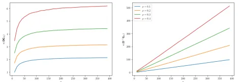
Example I.13. Consider again the matrixD from

Exam-ple I.1. Forρ∈{0.1, 0.2, 0.3, 0.4} and n ranging from 1 to

400, m= bρn_c, we plot the average condition number κ(DG), whereG∈Rn×m is a Gaussian random matrix. As

Fig. 2: Condition numberκ(GmD)for the matrixD from Example I.1, and for its inverse.Gm is the projection to the firstm_{= bρ}n_ccoordinates of a Gaussiann_×n matrix

G

As we saw in Example I.1, the operator norm ofD is bounded by kσk∞≤2. The Frobenius norm, on the other

hand, is easily seen to bekDkF= kσk2=

p

2n₋1. Setting

m_=ρn, the condition number thus concentrates on a value bounded by

p

2n−1+2pm

p

2n₋1₋2pm≈ 1+p

2ρ

1−p

2ρ,

which is sensible ifρ<1/2. We remark that, by construc-tion, the bounds are not sharp, and also do not apply to the inverse D−1.

1) A note on applicability: The previous discussion has shown that the condition number bounds need only consider the restricted condition number of a random projection of a matrix, rather than the full matrix condition. However, as the bounds are multiplicative, even small values (for example,2) lead to bounds for the the statistical dimension of the transformed cone that may not be practical. In addition, the statistical dimension of the reference cone also determines how small the projected dimension m is allowed to become, further limiting the amount of potential reduction in condition. If, for example,

C is the descent cone of the`1-norm, then the resulting

bounds can only be used for the descent cones of the `1-norm at very sparse vectors. The same applies when

considering, instead of the difference matrix D and its inverse, diagonal matrices with various forms of decay in the entries (this corresponds to a version of weighted `1

recovery). In these cases, the expected condition of the randomly projected matrices can be improve dramatically, but still not enough to give non-trivial bounds across all sparsity levels. This limitation is inherent to the notion of condition number: Condition bounds are, by definition, pessimistic. In numerical analysis, they measure the worst case sensitivity of a problem to perturbations in the input. As such, it would be unrealistic to expect condition bounds to be able to accurately locate the statistical dimension of the descent cone of a composite regularizer, unless the matrixD involved is close to orthogonal.

2) A note on distributions: The results presented are based on integral geometry, and as such depend crucially onQ being uniformly distributed in the orthogonal group with the Haar measure. By known universality results [30], the results are likely to carry over to other distributions.

In the context of this paper, however, we are neither interested in actually preconditioning the matrices in-volved, nor are we using them as a model for observation or measurement matrices as is common in compressive sensing. The randomization here is merely a technical tool to improve bounds based on the condition number, and the question of whether this is a “realistic” distribution is of no concern.

E. Organisation of the paper

In Section II we introduce the setting of conically restricted linear operators, the biconic feasibility problem, and Renegar’s condition number in some detail. The characterization of this condition number in the generality presented here is new and of independent interest. Sec-tionIIIderives the main condition bound. In SectionIVwe change the scene and give a brief overview of conic integral geometry, culminating in a proof of TheoremBin SectionV. Finally, in SectionVIwe translate the results to the setting of convex regularizers. Appendix A presents some more details on the biconic feasibility problem, while Appendix B presents a general version of Gordon’s inequality. While this version is more general than what is needed in this paper, it may be of independent interest.

II. CONICALLY RESTRICTED LINEAR OPERATORS

In this section we discuss the restriction of a linear operator to closed convex cones and discuss Renegar’s condition number in some detail.

A. Restricted norm and restricted singular value

Before discussing conically restricted operators in more detail, we record the following simple but useful lemma, which generalizes the relation kerA=(imAT)⊥_.

Lemma II.1. Let D _⊆Rm be a closed convex cone. Then

the polar cone is the inverse image of the origin under the projection map,D◦_:={z∈Rm_:

〈y,z〉 ≤0for all y∈D}₌ Π−1

D(0). Furthermore, if A∈R

m×n_{, then}

A−1(D◦)=¡

ATD¢◦

, (II.1)

whereA−1_(D◦_)={x∈Rn_:Ax

∈D◦_{}denotes the inverse image}

ofD◦ _{under A.}

Proof. For the first claim, note that _kΠD(z)k =

maxy∈D∩Bm_〈z,y_〉, andmax_y∈D∩Bm_〈z,y_{〉 =}0 is equivalent to

〈z,y〉 ≤0for all y∈D, i.e., z∈D◦.

For (II.1), let x∈A−1_(D◦_{) and y∈D. Then 〈x,A}T_y 〉 = 〈Ax,y〉 ≤0, as Ax∈D◦. Therefore, A−1(D◦)_⊆(ATD)◦. On the other hand, if v∈(ATD)◦ and y∈D, then 〈Av,y〉 = 〈v,ATy〉 ≤0, so that Av∈D◦ and hence,(ATD)◦⊆A−1(D◦).

The following proposition provides geometric conditions for the vanishing of the restricted norm or singular value.

Proposition II.2. Let A∈Rm×n, C⊆Rn and D ⊆Rm be

closed convex cones. Then the restricted norm vanishes, kAkC→D=0, if and only if C ⊆(ATD)◦. Furthermore, the

restricted singular value vanishes, σC→D(A)=0, if and only

ifC∩(ATD)◦6={0}, which is equivalent to AC∩D◦6={0}or kerA∩C6={0}.

Proof. Using LemmaII.1 we haveΠD(Ax)=0if and only if Ax∈D◦. This shows_kAkC→D=0 if and only if Ax∈D◦ for all x∈C∩Sn−1, or equivalently,C⊆A−1(D◦)=(ATD)◦

by (II.1). The claim about the restricted singular value follows similarly: σC→D(A)=0if and only if Ax∈D◦ for some x∈C∩Sn−1, or equivalently,C∩A−1(D◦)6={0}. Ifx∈

C∩A−1(D◦) \ {0}, then either Ax is nonzero orx lies in the kernel of A, which shows the second characterization.

It is easily seen that the restricted norm is symmetric kAkC→D= kATkD→C,

kAkC→D= max

x∈C∩Bm_y∈max_D∩Bn〈Ax,y〉

= max

y∈D∩Bn_x∈max_C∩Bm〈A

T

y,x〉

= kATkD→C.

(II.2)

Such a relation does not hold in general for the re-stricted singular value. In fact, in Section II-B we will see that, unless C ₌D _=Rn, the minimum of _σC→D(A) and_σD→C(−AT)is always zero, ifC andD have nonempty interior, cf. (II.5). And ifC orD is a linear subspace then σD→C(−AT)=σD→C(AT).

Remark II.3. In the caseC=Rn,D=Rm, withm≥n, one

can characterize the smallest singular value of A as the inverse of the norm of the (Moore-Penrose) pseudoinverse

of A:

σ(A)= kA†k−1.

Such a characterization doesnot hold in general for the restricted singular value, i.e., in general one cannot write σC→D(A)as kA†k−_D1_→C. Consider for example the caseD= Rm _{andC a circular cone of angleαaround some center}

p∈Sn−1. Both cones have nonempty interior, but lettingα go to zero, it is readily seen thatσC→D(A)tends tokApk, whilekA†kD→C tends tokpTA†k, which is in general not equal to kApk−1, unless ATA=In.

B. The biconic feasibility problem

The convex feasibility problem in the setting with two nonzero closed convex cones C⊆Rn, D⊆Rm is given as:

∃x∈C\ {0} s.t. Ax∈D◦, (P) ∃y∈D\ {0} s.t. ₋ATy∈C◦. (D)

Using Lemma II.1 and Proposition II.2 we obtain the following characterizations of the primal feasible matrices P(C,D) :₌{A∈Rm×n:(P) is feasible},

P(C,D)(II.1=)©

A∈Rm×n:C∩¡

ATD¢◦

6={0}ª

[Prop.II.2]

= {A∈Rm×n:σC→D(A)=0}.

(II.3)

By symmetry, we obtain for the dual feasible matrices D(C,D) :={A∈Rm×n:(D) is feasible},

D(C,D)={A∈Rm×n:D_∩(−AC)◦6={0}} ={A∈Rm×n:σD→C(−AT)=0}.

(II.4)

In fact, we will see that σC→D(A)and σD→C(−AT)can be characterized as the distances to P(C,D) and D(C,D), respectively. We defer the proofs for this section to Appendix A.

In the following proposition we collect some general properties ofP(C,D)andD(C,D).

Proposition II.4. LetC⊆Rn,D⊆Rmbe closed convex cones with nonempty interior. Then

1) P(C,D)andD(C,D) are closed; 2) the union of these sets is given by

P(C,D)_∪D(C,D)₌

(

{A∈Rm×n: detA=0} C=D=Rn Rm×n _else;

3) the intersectionP(C,D)∩D(C,D)is nonempty but has Lebesgue measure zero.

Note that from (2) and the characterizations (II.3) and (II.4) ofP(C,D)andD(C,D), respectively, we obtain for every A ∈ Rm×n: min{σC→D(A),σD→C(−AT)} = 0 or, equivalently,

max©

σC→D(A),σD→C(−AT)

ª

=σC→D(A)+σD→C(−AT), (II.5) unlessC₌D₌Rn.

In the following we simplify the notation by writing P,_D instead of_P(C,D),_D(C,D). For the announced inter-pretation of the restricted singular value as distance to P,D we introduce the following notation: for A∈Rm×n define

dist(A,P) :=min{k∆k:A+∆∈P}, dist(A,D) :=min{k∆k:A+∆∈D},

where as usual, the norm considered is the operator norm. The proof of the following proposition, given in Appendix A, follows along the lines of similar derivations in the case with a cone and a linear subspace [31].

Proposition II.5. LetC_⊆Rn,D_⊆Rmnonzero closed convex

cones with nonempty interior. Then

dist(A,P)=σC→D(A),

dist(A,D)₌σD→C(−AT).

We finish this section by considering the intersection ofP andD, which we denote by

or simply _Σwhen the cones are clear from context. This set is usually referred to as the set of ill-posed inputs. As shown in Proposition II.4, the set of ill-posed inputs, assumingC_⊆Rn andD_⊆Rmeach have nonempty interior, is a nonempty zero volume set. In the special caseC₌Rn,

D₌Rm,

Σ(Rn,Rm)={rank deficient matrices in Rm×n_}. From (II.5) and Proposition II.5 we obtain, if (C,D)6= (_Rn,_Rn),

dist(A,Σ)₌max©

dist(A,P), dist(A,D)ª

=dist(A,P)+dist(A,D).

The inverse distance to ill-posedness forms the heart of Renegar’s condition number [32], [14]. We denote

RC,D(A) := k

Ak dist(A,Σ(C,D))

=min

½

kAk σC→D(A)

, kAk σD→C(−AT)

¾

.

(II.6)

Furthermore, we abbreviate the special caseD_=Rm, which corresponds to the classical feasibility problem, by the notation

RC(A) :=RC,Rm(A). (II.7)

Note that the usual matrix condition number is recovered in the case C=Rn, D=Rm,

RRn(A)₌RRn_,Rm(A)₌κ(A).

Another simple but useful property is the symmetry RC,D(A)=RD,C(−AT). Finally, note that the restricted singular value has the following monotonicity properties

C⊆C0⇒σC→D(A)≥σC0_→D(A),

D_⊆D0_⇒σC→D(A)≤σC→D0(A).

This indicates that not necessarilyRC(A)≤RC0(A)ifC⊆C0.

But in the caseC0=Rn andm≥nthis inequality does hold, which we formulate in the following lemma.

Lemma II.6. LetC_⊆Rn closed convex cone with nonempty

interior and A∈Rm×n withm_≥n. Then

RC(A)≤κ(A). (II.8)

Proof. In the caseC=Rn we haveRRn(A)=κ(A). IfC6=Rn

then AC_6=Rm, asm_≥n. It follows thatRm

∩(−AC)◦6={0}, and thus_σRm_→C(−AT₎₌₀, cf. (II.4). Hence,

RC(A)= k

Ak σC→Rm(A)≤

kAk

σRn_→Rm(A)=κ(A).

To conclude this section, we state a useful bound on the condition number of a product of matrices.

Lemma II.7. Let A∈Rm×n withm≤n and letB∈Rm×m

be nonsingular. Then

RC(B A)≤κ(B)·RC(A).

Proof. We need to bound the numerator from above and the denominator from below in the definition of Regenar’s condition number (II.6). For the norms we have kB Ak ≤

kBk·kAk. If_σC(B A)=σRm_→C(−ATBT₎₌₀, then clearly also

σC(A)=σRm_→C(₋AT)₌0. Assume that σ_C(B A)₆₌0, and

let x∈C_∩Sn−1_{. Since B is non-singular, Ax}

6=0 and set

z=Ax/kAxk. Then

kB Axk = kB zk · kAxk ≥σ(B)·σC(Ax)6=0.

IfσRm_→C(−ATBT)6=0, then ifx∈Sm−1andz=BTx/kBTxk,

then

kΠC(ATBTx)k = kΠC(ATz)k · kBTxk ≥σ(B)_·σRm_→C(₋AT)₆₌0.

The condition bound follows.

III. LINEAR IMAGES OF CONES

The norm of the projection is a special case of a cone-restricted norm:

kΠC(g)k = kgkR+→C, (III.1)

where on the right-hand side we interpret g ∈Rn×1 as linear map fromRto Rn_{. In this section we relate these} norms for linear images of convex cones. The upper bound in TheoremIII.1is a special case of a more general bound for moment functionals [28, Proposition 3.9].

Theorem III.1. LetC ⊆Rn be a closed convex cone, and

νr(C) :=E[kΠC(g)kr], with g ∈Rn Gaussian. Then for A∈ Rp×n_{, andr}

≥1,

νr(AC)≤RC(A)rνr(C). (III.2)

In particular, if p≥n and Ahas full rank, then δ(C)

κ(A)2≤δ(AC)≤κ(A)

2_{δ(C). (III.3)}

The proof of Theorem III.1 relies on the following auxiliary result, LemmaIII.2, and on a generalized form of Slepian’s inequality, TheoremIII.3.

Lemma III.2. LetC_⊆Rn be a closed convex cone and A∈

Rp×n_{. Then}

1

kAkA(C∩B n₎

⊆AC_∩Bp_{⊆ λ}1A(C_∩Bn), (III.4)

withλ:=max©

σC→Rp(A),σ_Rp_→C(−AT)ª.

Proof. For the lower inclusion, note that any y∈A(C_kA∩kBn)

can be written asy=_kAx_Ak, withx∈C∩Bn. SincekAxk ≤ kAk, we have y∈convn0,_kAx_Axko⊂(AC)∩Bp. which was to be shown.

For the upper inclusion, let λ1 := σC→Rp(A), λ₂ :=

σRp_→C(−AT). We show in two steps thatAC∩Bp ⊆ 1

λ1A(C∩

Bn)ifλ1>0 and AC∩Bp ⊆_λ1₂ A(C∩Bn)ifλ2>0.

(1) Let_λ1>0. Since AC∩Bpas well as A(C∩Bn)contain

the origin, it suffices to show that AC_∩Sp−1

⊆_λ1₁ A(C_∩Bn). Every element inAC_∩Sp−1can be written as_kAy0_Ay0kfor some

y0∈C∩Sn−1, and since σC→Rp(A)₌min_y

∈C∩Sn−1kAyk ≤ kAy0k, we obtainσC→Rp(A) Ay0

kAy0k∈conv{0,Ay0}⊆A(C∩B

n_).

(2) Let_λ2>0. Recall from (II.4) thatλ2=σRp_→C(−AT_)>

0 only if (AC)◦_{={0}, i.e., AC=R}p_{. Observe that}

σRp_→C(−AT)= min

z∈Sp−1y∈maxC∩Bn〈Ay,z〉

=max©

r_≥0 :r Bp_⊆A(C_∩Bn)ª

.

This showsBp⊆_λ1₂ A(C∩Bn)and thus finishes the proof.

The following generalization of Slepian’s inequality is the special case of a generalized version of Gordon’s inequality for Gaussian processes, [28, Theorem B.2], when settingm=1 in that theorem.

Theorem III.3. Let Xj,Yj, j∈{0, . . . ,n}, be centered

Gaus-sian random variables, and assume that for all j,k≥0 we have

E|Xj−Xk|2≤E|Yj−Yk|2.

Then for any monotonically increasing convex function f:_R+→R,

Emax

j f+(Xj−X0)≤Emaxj f+(Yj−Y0), (III.5)

where f₊(x) :=f(x), ifx≥0, and f₊(x) :=f(0), ifx≤0.

Proof of TheoremIII.1. Set λ :₌ max©

σC→Rp(A),σ_Rp_→C(₋AT)ª. For the upper bound,

note that by Lemma III.2we have

E[kΠAC(g)kr]=E

·

max x∈AC∩Bp〈g,x〉

r¸ ≤ 1

λr E

·

max

x∈C∩Bn〈g,Ax〉

r¸_. Letg be a standard Gaussian vector and consider the Gaus-sian processes Xx= 〈g,Ax〉 andYx= 〈g,kAkx〉, indexed by x∈C∩Bn. For anyx,y∈C∩Bn we have

E(Xx−Xy)2= kAx−Ayk2≤ kkAkx− kAkyk2=E(Yx−Yy)2,

we get_E(Xx−Xy)2≤E(Yx−Yy)2. From Theorem III.3we conclude that for any finite subset S_⊂C_∩Bn containing the origin,

E[max x∈S X

r

x]≤E[max x∈S Y

r x].

By a standard compactness argument (see, e.g., [1, 8.6]), this extends to the whole index setC_∩Bn, which yields the inequalities

νr(AC)=E[kΠAC(g)kr]

≤ 1 λrE

·

max

x∈C∩Bn〈g,Ax〉

r

¸

≤kAk r

λr E

·

max x∈C∩Bn〈g,x〉

r

¸

=RC(A)rνr(C).

The upper bound in terms of the usual matrix condition number follows courtesy of (II.8). The lower bound proceeds along the lines, with the roles of _kAk and λ reversed. More specifically, from Lemma III.2we get the inequality

E[kΠAC(g)kr]≥

1 kAkrE

·

max

x∈C∩Bn〈g,Ax〉

r¸_.

Define

σC−C(A)= min z∈S(C−C)kAzk,

whereS(C−C) :={(x−y)/kx−yk:x∈C∩Bn,y∈C∩Bn,x6=y}. Consider the processesYx= 〈g,Ax〉andXx= 〈g,σC−C(A)x〉 indexed by x∈C∩Bn. Then for distinctx,y∈C∩Bn,

E(Xx−Xy)2= kσC−C(A)x−σC−C(A)yk2 ≤ kAx−Ayk2=E(Yx−Yy)2.

We can now apply Slepian’s inequality as we did for the upper bound, and conclude that

E[_kΠAC(g)kr]≥σC−C

(A)r kAkr νr(C).

To finish the argument, note that we have_σC−C(A)≥σ(A).

IV. CONIC INTEGRAL GEOMETRY

In this section we use integral geometry to develop the tools needed for deriving a preconditioned bound in Theorem B. A comprehensive treatment of integral geometry can be found in [33], while a self-contained treatment in the setting of polyhedral cones, which uses our language, is given in [34].

A. Intrinsic volumes

The theory of conic integral geometry is based on the

intrinsic volumesv0(C), . . . ,vn(C)of a closed convex cone

C_⊆Rn. The intrinsic volumes form a discrete probability distribution on {0, . . . ,n}that capture statistical properties of the coneC. For a polyhedral coneC and 0≤k≤n, the intrinsic volumes can be defined as

vk(C)=P{ΠC(g)∈relint(F), dimF=k},

where F is a face of C and relint denotes the relative interior.

Example IV.1. Let C ₌L_⊆Rn be a linear subspace of

dimensioni. Then

vk(C)=

(

1 if k₌i, 0 if k₆₌i.

Example IV.2. LetC=Rn_≥0 be the non-negative orthant,

i.e., the cone consisting of points with non-negative coordinates. A vector x projects orthogonally to a k -dimensional face ofC if and only if exactly k coordinates are non-positive. By symmetry considerations and the invariance of the Gaussian distribution under permutations of the coordinates, it follows that

vk(Rn_≥0)=

Ã

n k

!

2−n.

For non-polyhedral closed convex cones, the intrinsic volumes can be defined by polyhedral approximation. To avoid having to explicitly take care of upper summation bounds in many formulas, we use the convention that

convention follows from the fact that intrinsic volumes are “intrinsic”, i.e., not dependent on the dimension of the space in whichC lives).

The following important properties of the intrinsic vol-umes, which are easily verified in the setting of polyhedral cones, will be used frequently:

(a) Orthogonal invariance. For an orthogonal

transfor-mationQ∈O(n),

vk(QC)=vk(C);

(b) Polarity.

vk(C)=vn−k(C◦);

(c) Product rule.

vk(C×D)=

X

i+j=k

vi(C)vj(D). (IV.1)

In particular, ifD₌Lis a linear subspace of dimension

j, thenvk+j(C×L)=vk(C).

(d) Gauss-Bonnet.

n

X

k=0

(−1)kvk(C)=

(

0 ifC is not a linear subspace,

1 else.

(IV.2)

0 5 10 15 20 25

0 0.05 0.1 0.15 0.2 0.25 0.3 0.35

Fig. 3: Intrinsic volumes of the coneC={x:x1≤ · · · ≤xn}.

B. The statistical dimension

In what follows it will be convenient to work with reparametrizations of the intrinsic volumes, namely the tail and half-tail functionals

tk(C)=

X

i≥0

vk+i(C), hk(C)=2

X

i≥0even

vk+i(C),

which are defined for 0≤k ≤n. Adding (or subtract-ing) the Gauss-Bonnet relation (IV.2) to the identity

P

i≥0vi(C)=1, we see that h0(C)=h1(C)=1 if C is not

a linear subspace, so that the sequences 2v0(C), 2v2(C), . . .

and 2v1(C), 2v3(C), . . . are probability distributions in their own right. Moreover, we have the interleaving property

ti+1(C)≤hi(C)≤ti(C).

The intrinsic volumes can be recovered from the half-tail functionals as

vi(C)=

(₁

2(hi(C)−hi+2(C)) for0≤i≤n−2, 1

2hi(C) else.

(IV.3)

An important summary parameter is the statistical dimen-sion of a coneC, defined as the expected value of the intrinsic volumes considered as probability distribution:

δ(C)= n

X

k=0

kvk(C)=

1 2h1(C)+

X

i≥2 hi(C).

The statistical dimension coincides with the expected squared norm of the projection of a Gaussian vector on the cone,_δ(C)_=E£

kΠC(g)k2

¤

. Moreover, it differs from the squared Gaussian width by at most 1,

w2(C)≤δ(C)≤w2(C)+1,

see [7, Proposition 10.2].

The statistical dimension reduces to the usual dimension for linear subspaces, and also extends various properties of the dimension to closed convex conesC_⊆Rn:

(a) Orthogonal invariance.For an orthogonal

transfor-mationQ∈O(n),

δ(QC)=δ(C);

(b) Complementarity.

δ(C)+δ(C◦)=n; (IV.4)

This generalizes the relationdimL+dimL⊥=n for a linear subspaceL⊆Rn.

(c) Additivity.

δ(C×D)=δ(C)+δ(D).

(d) Monotonicity.

δ(C)_≤δ(D)ifC_⊆D.

The analogy with linear subspaces will be taken further when discussing concentration of intrinsic volumes, see SectionIV-D.

C. The kinematic formulas

The intrinsic volumes allow to study the properties of random intersections of cones via thekinematic formulas. A self-contained proof of these formulas for polyhedral cones is given in [34, Section 5]. In what follows, when we say that Q is drawn uniformly at random from the orthogonal groupO(d), we mean that it is drawn from the Haar probability measure ν onO(n). This is the unique regular Borel measure on O(n) that is left and right invariant (ν(QA)=ν(AQ)=ν(A)forQ∈O(n)and a Borel measurable A⊆O(n)) and satisfiesν(O(n))=1. Moreover, for measurable f :O(n)→R+, we write

EQ∈O(n)[f(Q)] :=

Z

Q∈O(n)

f(Q)ν(dQ)