warwick.ac.uk/lib-publications
Original citation:
Pollicott, Mark. (2016) A nonlinear transfer operator theorem. Journal of Statistical Physics,
166 (3). pp. 516-524.
Permanent WRAP URL:
http://wrap.warwick.ac.uk/82946
Copyright and reuse:
The Warwick Research Archive Portal (WRAP) makes this work of researchers of the
University of Warwick available open access under the following conditions.
This article is made available under the Creative Commons Attribution 4.0 International
license (CC BY 4.0) and may be reused according to the conditions of the license. For more
details see: http://creativecommons.org/licenses/by/4.0/
A note on versions:
The version presented in WRAP is the published version, or, version of record, and may be
cited as it appears here.
DOI 10.1007/s10955-016-1646-1
A Nonlinear Transfer Operator Theorem
Mark Pollicott1
Received: 22 June 2016 / Accepted: 18 October 2016 / Published online: 9 November 2016 © The Author(s) 2016. This article is published with open access at Springerlink.com
Abstract In recent papers, Kenyon et al. (Ergod Theory Dyn Syst 32:1567–15842012), and Fan et al. (C R Math Acad Sci Paris 349:961–9642011, Adv Math 295:271–3332016) introduced a form of linear thermodynamic formalism based on solutions to a non-linear equation using matrices. In this note we consider the more general setting of Hölder continuous functions.
Keywords Ruelle operator theorem·Transfer operator·Thermodynamic formalism
1 Introduction
We first recall a classical result for matrices dating back to work of Perron (1907) and Frobenius (1912) (cf. [5], p. 53). Ak×kmatrix Ais callednon-negativeif all the entries are non-negative real numbers andaperiodicif there existsn>0 such that all entries of the
nth powerAnare strictly positive.
Theorem 1.1 (Perron–Frobenius Theorem)Let A be a non-negative aperiodic k×k-matrix. There exists a unique positive maximal eigenvalueλ >0and a unique positive eigenvector vsuch that Av=λv.
We next recall a generalisation of the Perron–Frobenius Theorem to Banach spaces of functions. Letσ : → be a one-sided mixing subshift of finite type with alphabet
F = {1,· · ·,k}(i.e., there exists an aperiodick×kmatrix Bwith 0–1 entries such that
= {x = (xn)∞n=0 ∈ ∞
n=0F:xn ∈ F,B(xn,xn+1) = 1,∀n ≥0}and(σx)n = xn+1.
Given 0< θ <1, letFθbe the space of functions f :→Rfor which the semi-norm
Dedicated to David Ruelle on the occasion of his 80th Birthday.
B
Mark PollicottA Nonlinear Transfer Operator Theorem 517
fθ =sup
n≥0
varn(f) θn <+∞
is finite, where varn(f)=sup{|f(x)−f(x)|:xi=xifori=0,· · ·,n−1}. In particular, Fθis a Banach space with respect to the normf = fθ+ f∞.
Definition 1.2 Letφ∈Fθ. We can define a transfer operatorLφ:Fθ →Fθby
Lφψ(x)=
σy=x
eφ(y)ψ(y),
whereψ∈Fθandx∈.
The following result of Ruelle is a cornerstone of the classical theory of thermodynamic formalism (cf.[10]).
Theorem 1.3 (Ruelle–Perron–Frobenius Theorem)Letφ∈Fθ.
1. There existsλ=λφ>0andϕ=ϕφ ∈Fθwithψ >0such thatLφϕ=λϕ;
2. anyψ∈FθwithLφψ=λψis necessarily a multiple ofψ; and
3. the dependencesFθ φ→λφ ∈R+andFθ φ→ϕφ∈Fθare analytic.
It is also known that, aside from the maximal eigenvalueλ, the rest of the spectrum of
Lφ :Fθ →Fθis contained in{z∈C:|z|< λφ}. In particular, part 3 of Theorem1.3then follows from part 1 by standard perturbation theory.
The valueP(φ):=logλφis called thepressureof the functionφ∈Fθ[10]. In the case thatφ(x) = φ(x0,x1)depends only on the first two terms inx = (xn)∞n=0then Theorem
1.3reduces to Theorem1.1, by taking A(i,j) = expφ(i,j). In this case,ψ(x) =ψ(x0)
depends only on the first term and we can setv=(ψ(1), . . . , ψ(k)).
Recently, several authors introduced a particular non-linear version of Theorem1.1for matrices which is useful in the study of the dimension of certain sets in the theory of non standard ergodic averages (see section2).
Theorem 1.4 (Kenyon–Peres–Solomyak, Fan–Schmeling–Wu)Let B be a non-negative irreducible k×k matrix. There exists a unique positive vectorvsuch that Bv=v2, where the entries ofv2are the square of those ofv, i.e.,(v)
i2=vifor i=1,· · ·,k.
In the special case thatAhas entries which are natural numbers, this appears as Lemma 1.2 in [6]. A version of this for more general positive matrices appears as 4.1 in [2] (cf. also [3]) under very modest assumptions on the matrix. Other types of non-linear Perron–Frobenius Theorem appear in [7] and [8].
The following is our main result, which can be viewed either as a non-linear version of Theorem1.3, or a generalisation of the Theorem1.4(at least for aperiodic matrices) from matrices to functions.
Theorem 1.5 (Main Theorem)Letφ∈Fθ.
1. There existsψ=ψφ ∈Fθwithψ >0such thatLφψ=ψ2; 2. for anyψ∈FθwithLφψ=ψ2andψ>0thenψ=ψ;and
0.0 0.2 0.4 0.6 0.8 1.0 0.0
0.2 0.4 0.6 0.8 1.0 1.2
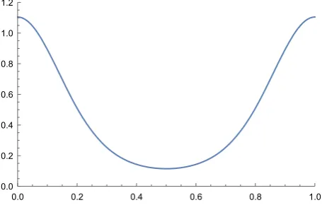
Fig. 1 A plot ofψφ(x)using the dyadic expansion 0≤∞n=0(xn−1)
2n+1 ≤1 on the unit interval to represent
x∈2
The result easily generalises toLφψ =ψq, for any natural numberq≥2. We consider only the caseq=2 to avoid introducing additional notation.
In the particular case that the functionφ(x) =φ(x0,x1)depends on only finitely many
coordinates then Theorem1.4can be recovered as a corollary to Theorem1.5.
Example 1.6 Let2= {1,2}Z+correspond to a full shift withF= {1,2}. We can define a
functionφ:2→Rby
φ(x)= −4 sin
2π
∞
n=0
(xn−1)
2n+1
and observe thatφ ∈Fθ for any 1/2 < θ <1. By Theorem1.5(with the choiceq = 2) there is a functionψ such thatLφψ = ψ2. In Fig.1we plot a realisation ofψ using the
dyadic expansion on the unit interval.
Remark 1.7 Ifφ ∈Fθ then, as usual, by replacingφbyφ1 =φ+logψφ−logψφ◦σ ∈
Fθ, whereψ is the positive eigenfunction in Theorem1.3, we can assume without loss of generality thatψφ1(x) = 1is the constant function taking the value 1, i.e.,Lφ11 = λ1, whereλ=λφ =λφ1. In particular, for such special normalized functionsφ1 the function
ψTheorem1.5can easily be identified asψ =ψφ1 = λ1, then we see thatLφ1ψ = ψ2.
Furthermore, the hypothesis for analyticity in part 3 of Theorem1.5automatically holds.
I am grateful to the referees and the editors for their patience and help with this short note.
2 Background to Theorem
1.4
Although our main result (Theorem1.5) is of independent interest, for the reader’s benefit we will now give a brief description of the original application of its precursor (Theorem1.4) which provided the motivation for its introduction.
[image:4.439.106.334.57.202.2]A Nonlinear Transfer Operator Theorem 519
partition ofNbyN= ∪joddj. We can then defineν=
jμ, in a natural sense. In [6]
and [3] the authors consider the measureμto be a (generalised) Markov measure defined in terms of the entries in the vectorvin Theorem1.4. The measureνwill typically not be
σ-invariant but is still useful in studying the Hausdorff dimension of certain sets. We can define the pointwise dimension ofνby
dimH(ν)= − lim
n→+∞
1
nlogν ([x0,x1,· · ·,xn−1]) for a.e.(ν)x=(xn)∈
where[x0,x1,· · ·,xn−1] = {y = (yn) ∈ :xi = yi,0 ≤ i ≤n−1}is a cylinder set.
Finally, by Proposition 2.3 of [6] we have that for anyσ-ergodic measureνthe pointwise dimension is constant and takes the explicit value
dimH(ν)=
∞
n=1
1 2n+1Hμ
∨n−1
i=0σ−iα
whereα = {[1], . . . ,[k]}is the standard partition into cylinders of length one;∨ni=−01σ−iα is the usual refinement to a partition by cylinders of lengthn; andHμ(·)is the entropy for partitions [11].
The pointwise dimension is particularly useful in estimating the Hausdorff Dimension of sets (especially lower bounds via the usual mass distribution principle cf. [1], §4.2) associated to multiple ergodic theorems, as the following example illustrates.
Example 2.1 (Golden Mean Example [4,6]) Fan–Liao–Ma and Kenyon–Peres–Solomyak considered the golden mean example:
X= (xn)∈ {0,1}N:xnx2n =0,∀n≥1
,
with the usual metric
dθ(x,x)=
θN(x,x) ifx =x
0 ifx =x.
whereN(x,x)=sup{n≥0 :xi =xifor 0≤i≤n}(andN(x,x)=0 ifx0=x0).
In this case one can consider the matrix B=
1 1 1 0
and the solution to Bv =v2, i.e.,
v=
v1
v2
satisfiesv21 =v1+v2andv22=v1. We then have thatμis a Markov measure for
P=
p 1−p
1 0
, wherep3=(1−p)2, and finally dimH(X)= −log2p=0·81137. . .
which is strictly less than the Minkowski dimensiondi mM(X)=0·82429. . .[4,6].
3 Proof of Theorem
1.5
3.1 Existence of the Fixed Point
The existence can be shown by looking for a fixed point of a suitable map in the space
c:= u:→ [0,1]:u(x)≤u(x)ecdθ(x,x
)
for thosex,x∈withx0=x0
wherec>0 anddθ(·,·)is as defined in Example2.1. We first note thatc ⊂Fθsince for
u∈candx,x∈we can boundu(x)−u(x)≤ u∞
ecdθ(x,x)−1≤Cd θ(x,x)
for sufficiently largeC >0 and then interchangingx andxgives thatuθ ≤C (cf. [9], p. 22).
We can now introduce a family of non-linear operators defined as follows:
Definition 3.1 For eachn≥1 we can associate tou∈ca new functionNn(u):→R
defined by
Nn(u)(x)=
Lφu+1n1(x)
Lφu+1n1∞
1 2
where1n1represents the function taking the constant value 1n.
Lemma 3.2 We have thatLφ(c)⊂c for c=(c+ φθ)θ.
Proof Letx,x ∈ withx0 = x0. Assume thatdθ(x,x) = θN, for some N ≥ 0, then
xi =xifor 0≤i ≤N andxN+1 =xN+1. Ify ∈σ−1x then we denote byy∈σ−1xthe
corresponding sequence for whichy0 = y0, and thus we have thatdθ(y,y) =θN+1. Let
u∈cthen we have that
Lφu(x)=σy=xeφ(y)u(y)
≤σy=xeφ(y
)+φθθN+1
u(y)ecθN+1
≤e(c+φθ)θdθ(x,x)
σy=xeφ(y
)
u(y)
=e(c+φθ)θdθ(x,x)L φu(x)
where we have used thatdθ(y,y) = θN+1 and then sinceu ∈ cwe have thatu(y) ≤ u(y)ecθN+1
. In particular, we have thatLφu(x)≤ecdθ(x,x)Lφu(x), i.e.,Lφu∈
c.
Remark 3.3 By definition ofc, we see that ifc <cthenc ⊂cthus, providingcis
sufficiently large, Lemma3.2givesLφ(c)⊂c.
We can use the above lemma to deduce the following.
Lemma 3.4 For c>0sufficiently large we have thatNφ(c)⊂c.
Proof Letu∈c. For eachn≥1 the constant function1n1∈cand so by applying Lemma 3.2to the new functionu+n11we see that
Lφ
u+1 n1
(x)≤ecdθ(x,x)L φ
u+ 1 n1
(x), (3.1)
for allx,x ∈ withx0 = x0. Dividing both sides of (3.1) byL
u+ 1n1∞ >0 we have that
Lφu+1n1(x)
Lu+1n1∞ ≤e
cdθ(x,x)Lφ
u+1n1(x)
A Nonlinear Transfer Operator Theorem 521
Finally, since the values taken by both sides of (3.2) lie in the unit interval, taking square roots preserves this property withcreplaced byc/2, i.e.,
Nn(u)(x)=
Lφ
u+1n1
(x)
Lφ
u+1
n1
∞ 1
2
≤e(c/2)dθ(x,x)
Lφ
u+1n1
(x)
Lφ
u+1
n1
∞ 1
2
=e(c/2)dθ(x,x)N n(u)(x)
i.e.,Nn(u)∈c/2. Providingcis sufficiently large thatc>c/2=(c+ φθ)θ/2 we have
thatc/2⊂cand the result follows.
This now brings us to the existence of the fixed point for each of the operatorsNn:c→ c.
Lemma 3.5 For each n ≥ 1, there exists a non-trivial fixed pointψn ∈ c such that Nn(ψn)=ψn.
Proof By the Arzela–Ascoli Theorem the spacecis compact with respect to the norm·∞.
For eachn≥1 andc>0 sufficiently large the mapNn :c→cis a continuous map on
a compact convex subspace ofC0()and we can apply the Schauder fixed point theorem to deduce that there is a fixed pointψn ∈cforNn. To see thatψnis not identically zero we
need only observe that by the definition ofNnthere existsx(n)∈withNn(ψn)(x(n))=1
and by constructionψn(x(n))=Nn(ψn)(x(n))=1. This completes the proof.
We can now use the compactness ofcwith respect to · ∞to deduce that(ψn)∞n=1
has a · ∞-convergent subsequence. We denote the limit point byψ0∈and observe that
we have thatLφ(ψ0)=λψ02, whereλ= Lφ(ψ0)∞. Moreover, since we observed that by
construction thatψn∞=1, for eachn≥1, we can deduce thatψ0∞=1 and thus, in
particular,ψ0is non-zero. If we replaceψ0byψ =λψ0then we finally getLφ(ψ)=ψ2,
as required.
To see thatψ >0, assume for a contradiction that there existsx0∈such thatψ(x0)=0.
Sinceψ ≥ 0 we see from the identityLφ(ψ)(x0) = ψ2(x0) = 0, which implies that
ψ(y) = 0 wheneverσy = x0. Proceeding iteratively, we have thatψ vanishes on the set
∪∞
n=0σ−nx0, which is dense by the mixing hypothesis onσ:→(corresponding to the
aperiodicity assumption onA). However, this contradicts thatψ=0.
3.2 Uniqueness of the Positive Fixed Point
Assume for a contradiction that we had a second distinct non-trivial positive fixed point, i.e.,
Lφ(ψ)=ψ2withψ>0 andψ=ψ. We can then associateξ :=inf{t>0 :tψ−ψ≥
0}and thus, in particular,ξψ≥ψ. Observe thatLφ(ξψ−ψ)=ξψ2−ψ2 ≥0, sinceLφ preserves positive functions. Sinceξψ2−ψ2=(√ξψ+ψ)(√ξψ−ψ)≥0 we deduce
that√ξψ−ψ≥0. In particular, this implies thatξ ≤1, otherwise it contradicts the original definition ofξ.
Interchanging the roles ofψ andψwe can defineξ:=inf{t >0 :tψ−ψ ≥0}and and thus, in particular,ξψ ≥ψ ≥0. A similar argument to the above shows thatξ ≤1. However, since we can then write(ξξ)ψ≥ξψ≥ψthis implies thatξ =ξ=1.
For the definition of ξ we can choose x0 with ψ(x0) = ψ(x0). We can then write
Lφ(ψ−ψ)(x
0)= ψ2(x0)−ψ2(x0) =(ψ(x0)+ψ(x0))(ψ(x0)−ψ(x0))=0 which
implies that ψ(y) = ψ(y) wheneverσy = x0. Proceeding inductively we deduce that
ψ(y)=ψ(y)on the dense set ofy∈ ∪∞
Remark 3.6 This simple argument doesn’t rule out the possibility of another non-positive fixed point.
3.3 Analyticity
To show the analytic dependence of the solution we want to use the implicit function theorem applied to the functionG:Fθ×Fθ→Fθdefined by
G(φ, ψ)=Lφψ−ψ2.
In order to apply the implicit function theorem at(φ0, ψ0)∈ Fθ×Fθ withψ0 > 0, say,
satisfyingG(φ0, ψ0)=0 we need to show that(D2G)(φ0, ψ0):Fθ →Fθis invertible. An
easy calculation gives that
(D2G)(φ0, ψ0)=
Lφ0−2ψ0
:Fθ→Fθ. (3.3) The spectral radius of any linear operator is the radius of the smallest disk (centred at the origin) containing the spectrum.
We recall the following result [9] which is also due to Ruelle.
Lemma 3.7 (Ruelle)The operatorLφ0 :Fθ →Fθhas spectral radiusλφ0.
In particular, we see from Lemma3.7that(Lφ0 −2λφ01)−1 : Fθ →Fθ is a bounded linear operator since 2λφ0 is not in the spectrum ofLφ0. We can write
Lφ0−2ψ0
−1
=(Lφ0−2λφ0)1+2(λφ01−ψ0)
−1
=(Lφ0−2λφ01)−1
∞
n=0
2(λφ01−ψ0)(Lφ0−2λφ01)−1
n
which exists and is a bounded linear operator providedλφ01−ψ0< 2(Lφ 1
0−2λφ01)−1. In particular, by (3.3) we see that(D2G)(φ0, ψ0)is invertible and thus the implicit function
theorem applies. This allows us to deduce the analytic dependence.
Remark 3.8 (The Tangent Operator) Closely related to this circle of ideas is the use of a standard technique in understanding the iterates of a non-linear operator in a neighbourhood of a fixed point. More precisely, we consider the first order approximation toG(φ0,·):ψ →
Lφ0ψ −ψ
2 whereψ = ψ
0+ψ(1)+o(). A simple calculation gives that the tangent
operator
Tφ0ψ :=lim
0
G(φ0, ψ0+ψ(1))−G(φ0, ψ0)
=Lφ0ψ(
1)−2ψ 0ψ(1).
For definiteness, we can consider the specific case where we replaceφ0byφ1as in Remark1.7,
then we see that the spectra sp(Tφ1)and sp(Lφ1)are simply related by sp(Tφ1)=sp(Lφ1)−2. Thus, sinceλφ1=1, by Lemma3.7the tangent operatorTφ1will have its spectra in the disk centred at−2 and of radius 1 (and thus outside the unit disk, except for the value−1). This suggests that the fixed pointψφ1 is locally unstable in a codimension one space under the iterationG(φ1,·)n
4 Measures
The classical transfer operatorLφplays an important role in the ergodic theory of equilibrium states associated toφ. More precisely, the equilibrium state is a fixed point for the dualL∗φ
A Nonlinear Transfer Operator Theorem 523
to the transfer operatorLφ1(satisfyingLφ11=1) for the associated functionφ1(cf. Remark
1.6). Although there is no direct analogue of equilibrium states in the context of the nonlinear equationsLφψ =ψ2we have been studying, one can still use this identity to associate to
the two functionsφandψa natural invariant measure.
Given a solutionLφψ = ψ2 as in Theorem1.5, we can consider the linear operator
Mφ :Fθ→Fθgiven by
(Mφw)(x)=
σy=x eφ(y)
ψ ψ2◦σ
(y)w(y)
which then satisfiesMφ1 = 1 (cf. Remark1.7). SinceMφ is a transfer operator with a Hölder continuous potential, it is a consequence of the simplicity of the maximal positive eigenvalue for the operator in Theorem1.3, and thus of its dual, that there is a uniqueσ -invariant probability measureμsuch thatM∗φμ = μ, i.e., f dμ = Mψf dμfor all
f ∈C0(). This leads to a non-standard version of the variational principle.
Lemma 4.1 (Variational Principle forφandψ)For anyσ-invariant probability measureν we have that
h(ν)+φdν−logψdν≤0 (4.1)
with equality if and only ifν=μ.
Proof Letφ2:=φ+logψ−2 logψ◦σthen sinceMφ=Lφ2 satisfiesLφ21=1we see thatP(φ2)=0 andμis the unique equilibrium state associated toφ2, by Proposition 3.4 in
[9]. Thus by the variational principle (Theorem 3.5 in [9]) we have
h(ν)+(φ+logψ−2(logψ)◦σ )dν =h(ν)+φ2dν
≤P(φ2)=0=h(μ)+
φ2dμ
=h(μ)+(φ+logψ−2(logψ)◦σ )dμ
(4.2)
with equality if and only ifμ=ν. Byσ-invariance of the measures we have that(logψ)◦
σdμ=logψdμand(logψ)◦σdν=logψdνand thus (4.1) follows from (4.2).
We consequently have a particularly simple expression for the entropyh(μ).
Corollary 4.2 We can write
h(μ)=
(logψ)dμ−
φdμ.
Acknowledgements This work was supported by the Leverhulme Trust (RPG-2015-346) and EPSRC (EP/M0011903/1).
References
1. Falconer, K.: Fractal Geometry. Wiley, New York (1990)
2. Fan, A., Schmeling, J., Wu, M.: Multifractal analysis of multiple ergodic averages. C. R. Math. Acad. Sci. Paris349, 961–964 (2011)
3. Fan, A., Schmeling, J., Wu, M.: Multifractal analysis of some multiple ergodic averages. Adv. Math.295, 271–333 (2016)
4. Fan, A., Liao, L., Ma, J.: Level sets of multiple ergodic averages. Monatshefte für Mathematik168, 17–26 (2012)
5. Gantemacher, F.: The Theory of Matrices, vol. 2. American Mathematical Society, Providence (2000) 6. Kenyon, R., Peres, Y., Solomyak, B.: Hausdorff dimension for fractals invariant under the multiplicative
integers. Ergod. Theory Dyn. Syst.32, 1567–1584 (2012)
7. Krause, U.: Concave Perron-Frobenius theory and applications. In: Proceedings of the Third World Congress of Nonlinear Analysts, Part 3 (Catania, 2000). Nonlinear Analysis, vol. 47, no. 3, pp. 1457– 1466 (2001)
8. Lemmens, B., Nussbaum, R.: Nonlinear Perron-Frobenius Theory, Cambridge Tracts in Mathematics, vol. 189. Cambridge University Press, Cambridge (2012)
9. Parry, W., Pollicott, M.: Zeta functions and the periodic orbit structure of hyperbolic dynamics. Astérisque 187–188, 1–268 (1990)