Comparison of Several Data Mining Methods in Credit Card Default Prediction

ISSN Online: 2160-5920 ISSN Print: 2160-5912

DOI: 10.4236/iim.2018.105010 Sep. 26, 2018 115 Intelligent Information Management

Comparison of Several Data Mining Methods in

Credit Card Default Prediction

Shenghui Yang, Haomin Zhang

School of Science, Guilin University of Technology, Guilin, China

Abstract

LightGBM is an open-source, distributed and high-performance GB frame-work built by Microsoft company. LightGBM has some advantages such as fast learning speed, high parallelism efficiency and high-volume data, and so on. Based on the open data set of credit card in Taiwan, five data mining me-thods, Logistic regression, SVM, neural network, Xgboost and LightGBM, are compared in this paper. The results show that the AUC, F1-Score and the

predictive correct ratio of LightGBM are the best, and that of Xgboost is second. It indicates that LightGBM or Xgboost has a good performance in the prediction of categorical response variables and has a good application value in the big data era.

Keywords

LightGBM, Xgboost, AUC, F1-Score, Data Mining

1. Introduction

As an unsecured credit facility, credit cards have huge risks behind the high re-turns of banks. The ever-increasing number of credit card circulation cards has brought about an increase in the amount of credit card defaults, and the result-ing large amount of bills and repayment information data have also brought certain difficulties to the risk controllers. Therefore, how to use the data gener-ated by users, and extract useful information to control risks, reduce default rate, and control the growth of non-performing rate has become one of the key con-cerns of banks.

Credit card default prediction is based on the historical data of credit card customers. The use of corresponding methods to predict and analyze credit card customer default behavior is a typical classification problem. Data mining algo-How to cite this paper: Yang, S.H. and

Zhang, H.M. (2018) Comparison of Several Data Mining Methods in Credit Card De-fault Prediction. Intelligent Information Management, 10, 115-122.

https://doi.org/10.4236/iim.2018.105010 Received: August 28, 2018

Accepted: September 23, 2018 Published: September 26, 2018 Copyright © 2018 by authors and Scientific Research Publishing Inc. This work is licensed under the Creative Commons Attribution International License (CC BY 4.0).

http://creativecommons.org/licenses/by/4.0/

DOI: 10.4236/iim.2018.105010 116 Intelligent Information Management rithms have long been applied to the study of credit card default prediction problems. Thomas [1] used discriminant analysis to score the credits and beha-viors of borrowers; Yeh and Lien [2] used Logistic regression, decision trees, ar-tificial neural networks and other algorithms to predict customer default pay-ments in Taiwan, and compared the predictions of these algorithms. Accuracy, finally found that the correct rate of artificial neural network is slightly higher than the other five methods. Mei Ruiting, Xu Yang and Wang Guochang [3] ex-plored the key factors affecting customer credit by establishing Lasso-Logistic and random forest models. The results show that the accuracy of random forest prediction is higher than that of Lasso-Logistic.

2. Description of the Data

Feature Description

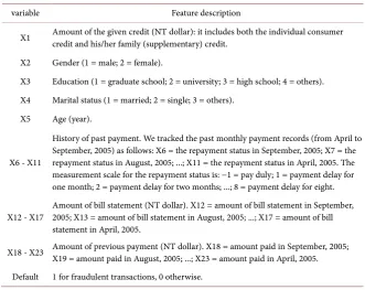
This article is based on credit card customer data from April to September 2005 in Taiwan on the UCI website. The data set contains 1 response variable (De-fault), 23 explanatory variables (X1 - X23), and 30,000 case data. The meaning of each variable in the data set is shown in Table 1. The frequency statistics of each category variable are shown in Table 1.

3. Introduction of the Method

3.1. Logistic Regression

Logistic regression is a special linear regression model. However, the two-category response variable violates the normal hypothesis of the general regression model.

Table 1. Default dataset of credit card.

variable Feature description

X1 Amount of the given credit (NT dollar): it includes both the individual consumer _{credit and his/her family (supplementary) credit.} X2 Gender (1 = male; 2 = female).

X3 Education (1 = graduate school; 2 = university; 3 = high school; 4 = others). X4 Marital status (1 = married; 2 = single; 3 = others).

X5 Age (year).

X6 - X11

History of past payment. We tracked the past monthly payment records (from April to September, 2005) as follows: X6 = the repayment status in September, 2005; X7 = the repayment status in August, 2005; ...; X11 = the repayment status in April, 2005. The measurement scale for the repayment status is: −1 = pay duly; 1 = payment delay for one month; 2 = payment delay for two months; ...; 8 = payment delay for eight.

X12 - X17 Amount of bill statement (NT dollar). X12 = amount of bill statement in September, 2005; X13 = amount of bill statement in August, 2005; ...; X17 = amount of bill statement in April, 2005.

DOI: 10.4236/iim.2018.105010 117 Intelligent Information Management The Logistic Regression Model specifies that the appropriate function of the event fit probability is a linear function of the observed values of the available explanatory variables. The main advantage of this approach is a simple classifi-cation probability formula can be generated. The insufficiency of Logistic re-gression is that the nonlinear and interactive effects of explanatory variables cannot be handled correctly.

3.2. Neural Network

Artificial neural networks use nonlinear mathematical equations to continuously establish meaningful relationships between input and output variables through the learning process. We apply backpropagation networks to classify data. Back-propagation neural networks use feedforward topology and supervised learning. The structure of a backpropagation network typically consists of an input layer, one or more hidden layers, and an output layer, each layer consisting of several neurons. Artificial neural networks can easily handle the nonlinearities and in-teractions of explanatory variables. The main disadvantage of artificial neural networks is that they do not give the result of a simple classification probability formula.

3.3. Support Vector Machine (SVM)

SVM is a pattern recognition method based on statistical learning theory. Which used the kernel function to map the data X of the input space into a high-di- mensional feature space, and then at high In the dimensional space, the genera-lized optimal classification surface is obtained, and then the data that is linearly inseparable in the original space can be linearly classified in the high-dimensional space. The main difficulty of SVM is that after the kernel function is deter-mined, when solving the problem classification, the quadratic programming of the solution function is required, which requires a large amount of storage space.

3.4. Xgboost

Boosting is a very effective integrated learning algorithm [4]. Boosting method can transform weak classification into strong classifier to achieve accurate classi-fication effect. The steps are as follows:

1) All the training set samples are given the same weight;

2) The mth iteration is performed, and each iterations is classified by a classi-fication algorithm, and the error rate

(

)

i i m i

m

i

I y G x err

ω

ω

≠ =

∑

∑

of the classification is calculated, wherein ωi represents the weight of the ith sample, I

( )

DOI: 10.4236/iim.2018.105010 118 Intelligent Information Management 4) for m+1 _{iteration, update the weight (}ω_{i) of the i sample:}

( )

m i m i

a I y G x i e

ω

(1) 5) After completing the iteration, all the classifiers are obtained, and the clas-sification result of each sample is obtained by voting. At its core, after each itera-tions, the sample with the wrong classification will be given a higher weight, thus improving the effect of the next classification.

Gradient Boosting (GB) is a kind of Boosting algorithm. It is proved that Boosting’s loss function is exponential, while GB is to make the loss function of the algorithm fall along its gradient direction during the iteration process, thus improving the robustness. The algorithm steps are:

1) 0

( )

(

)

1 arg minp N i,

i

f x L y γ

=

=

∑

2) For 1−m _iterations:

a) 0

( )

(

)

1 arg min_p N _i,

i

F x L y ρ

=

=

∑

b) m from 1 to M:

( )

(

)

( )

i _{F x F x}

L y F x

y i N

F x − = ∂  = −  = ∂    

 (2)

(

)

, 1

arg min N :

m i i m

i

a α β y βh X a

=

=

∑

( )

(

)

(

)

1

arg min N , :

m i m i i m

i L y F X h X a

ρ

ρ − ρ

=

=

∑

( )

( )

(

)

m m m i m

F X =F ₋ X +ρ h X a ₍₅₎

Xgboost is a fast implementation of the GB algorithm. It is a lifting algorithm based on decision tree. It takes both the linear model solver and the decision tree algorithm. The basic idea is to combine many decision tree models to form a model with high accuracy.

3.5. LightGBM

LightGBM is a gradient learning framework based on tree learning. The main difference between it and the Xgboost algorithm is that it uses a histogram-based algorithm to speed up the training process, reduce memory consumption, and adopt a leaf-wise leaf growth strategy with depth limitation [5]. The following describes the histogram algorithm and the leaf growth strategy with depth-limiting Leaf-wise.

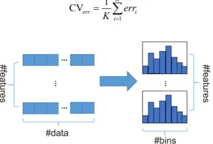
3.5.1. Histogram Algorithm

histo-DOI: 10.4236/iim.2018.105010 119 Intelligent Information Management gram accumulates the required statistic, and then traverses to find the optimal according to the discrete value of the histogram Split point. The process is shown in Figure 1.

3.5.2. Leaf-Wise Leaf Growth Strategy with Depth Limitation

The decision tree’s growth strategy is generally Level-wise, which is an inefficient algorithm because it treats the leaves of the same layer indiscriminately, result-ing in a lot of unnecessary memory consumption. Leaf-wise is a more efficient strategy. Every time from all the leaves, find the leaf with the highest split gain, then split and cycle. Therefore, compared with Level-wise, Leaf-wise can reduce more errors and get better precision when the number of splits is the same. The disadvantage of Leaf-wise is that it may grow a deeper decision tree and produce over-fitting. Therefore, LightGBM adds a maximum depth limit above Leaf-wise to prevent over-fitting while ensuring high efficiency. The leaf-wise leaf growth process is shown in Figure 2.

4. Evaluation Criteria

4.1. Model Test

K-fold cross-validation is a commonly used accuracy test method in machine learning. Its purpose is to obtain a reliable and stable model. In the general problem, when the response variable is a quantitative variable, the cross-validation uses the mean square error as an indicator to measure the test error. On the classification problem, when the response variable is a qualitative variable, cross-validation uses the CV error rate as a measure. The form of the K-fold CV error rate as follows:

1 1 CV_err K _i

i err

K =

=

∑

Figure 1. Ergodicity process of histogram algorithm.

DOI: 10.4236/iim.2018.105010 120 Intelligent Information Management

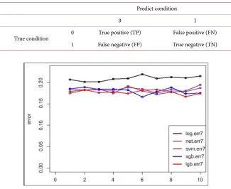
4.2. Classification Evaluation

Under normal circumstances, for the two classification labels 0 and 1, there are definitions as follows:

The expression of the Acc is defined as follow:

(

)

(

)

Acc

TP TN FP FN

+ =

+ + + (6)

Accuracy (Prec) and recall (Rec) are used to represent the general characteris-tics of the classifier. Accuracy is the percentage of cases that are marked as tive and indeed are indeed positive. The recall rate, also known as the true posi-tive rate, is the percentage of cases that should have been correctly identified as positive. According to Table 2, the accuracy and recall rate are expressed as fol-lows:

(

)

Prec

TP FP

=

+ (7)

(

)

Rec

TP FN

=

+ (8)

In general, Prec is high, Rec is low, Rec is high, and Prec is low. We need to balance the two and use F -scoreβ [6] to reconcile the two. Expressed as follows:

(

)

2

1 Prec Rec

F -score

Prec Rec β

β

β

+ ∗

=

+ (9)

In the case, Generally, when we think accuracy is more important, we set 0.5

β = ; if we think recall is more important, we set β=2. While β=1, we will get the harmonic mean value of the sum, which is recorded as the result of the sum, and the expression is as follows:

1 2 Prec Rec

F =

Prec Rec

∗ ∗

+ (10)

The relationship between the true positive rate and the false positive rate is called the ROC curve, and the ROC curve is used to verify the performance of a classifier model. The area under the curve (AUC) is a valid measure of the ROC curve and is an indicator of the comparison of different ROC curves.

5. Results

5.1. Ten Times Ten Fold Cross Validation Results

In this paper, ten times of ten-fold cross-validation is used to verify the model established by different data mining methods. The 10% CV error rate results are as follows:

DOI: 10.4236/iim.2018.105010 121 Intelligent Information Management Table 2. Confusion matrix.

Predict condition

0 1

True condition 0 True positive (TP) False positive (FN) 1 False negative (FP) True negative (TN)

Figure 3. The seventh times 10-fold CV error rate.

Table 3 shows the average 10% CV error rate of the five methods. It can be seen from Table 3 that the 10% CV error rate of the five methods is low, indi-cating the five data mining methods have certain reliability. The average 10% CV error rate difference between the five methods is small, but LightGBM’s 10 av-erage 10% CV error rate is slightly lower than the other four methods.

5.2. Classification Results

The classification results obtained from 10-fold cross-validation are shown in

Table 4.

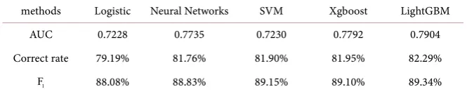
From Table 4 we can know that the accuracy rates of the five data mining methods are all above 79%, and the difference is not large. The correct rate of LightGBM is 82.29%, which indicates that these five methods have better classi-fication effects. AUC has a big difference. LightGBM has an AUC of 0.7904, and the other four methods have lower AUCs than LightGBM. At the same time, LightGBM is 89.34% higher than the other methods, indicating that LightGB has the best classification effect on the classification problem of this paper.

6. Conclusion

DOI: 10.4236/iim.2018.105010 122 Intelligent Information Management Table 3. The mean of 10 times 10-fold CV error rate.

methods Logistic _Networks Neural SVM Xgboost LightGBM The mean of 10 times

10-fold CV error rate 0.2091 0.1824 0.1810 0.1805 0.1771

Table 4. Comparison of model classification effect.

methods Logistic Neural Networks SVM Xgboost LightGBM

AUC 0.7228 0.7735 0.7230 0.7792 0.7904

Correct rate 79.19% 81.76% 81.90% 81.95% 82.29%

1

F 88.08% 88.83% 89.15% 89.10% 89.34%

cross-validation was performed to obtain the average AUC and correct rate of the model, and LightGBM was the highest among the three evaluation indica-tors, indicating that the data mining method has a good classification effect, and the classification effect is better than other four data mining methods.

Conflicts of Interest

The authors declare no conflicts of interest regarding the publication of this pa-per.

References

[1] Lyn, C. and Thomas, A. (2000) Survey of Credit and Behavioral Scoring: Forecast-ing Financial Risk of LendForecast-ing to Consumers. International Journal of Forecasting, 16, 149-172. https://doi.org/10.1016/S0169-2070(00)00034-0

[2] Yeh, I.-C. and Lien, C.-H. (2009) The Comparisons of Data Mining Techniques for the Predictive Accuracy of Probability of Default of Credit Card Clients. Expert Systems with Applications, 36, 2473-2480.

https://doi.org/10.1016/j.eswa.2007.12.020

[3] Mei, R.T., Xu, Y. and Wang, G.C. (2016) Analysis of Credit Card Default Prediction Model and Its Influencing Factors. Statistics and Application, 5, 263-275.

[4] Ye, Q.Y., Rao, H. and Ji, M.S. (2017) Business Sales Forecast Based on XGBOOST. Journal of Nanchang University, No. 3, 275-281.

[5] Guo, L.K., Qi, M., Finley, T., Wang, T.F., Chen, W., Ma, W.D., Ye, Q.W. and Liu, T.-Y. (2017) LightGBM: A Highly Efficient Gradient Boosting Decision Tree. 31st Conference on Neural Information Processing Systems (NIPS 2017), Long Beach, CA, USA, 4-9 December 2017, 1-9.