Credit risk modeling and CDS valuation
An analysis of structural models
Credit risk modeling and CDS valuation
An analysis of structural models
A thesis
submitted in partial fulfillment of the requirements for the degree of Master of Science
in Industrial Engineering and Management
University of Twente
by
Jeroen van Beem
Thesis Committee
Abstract
Preface
This is it. Although this preface might be the beginning of this master thesis for you, it is the end for me. It represents the end of long hours of working on this thesis, but also the end of my student time. A great time in which I made lots of friends and learned even more.
This thesis is written to obtain the degree of Master of Science in Industrial Engineering and Man-agement at the University of Twente. The eight months of research that I performed for this thesis at Deloitte Capital Markets were a great experience for me. It was an opportunity to broaden my knowledge and experience working in the financial services industry. Reviewing academic literature on credit risk, programming simulation models in Matlab and performing sensitivity analysis have been an interesting challenge. Now I look back at the project with satisfaction, knowing that I achieved my goals and produced useful results.
I would like to thank dhr. K. Dessens from Deloitte Capital Markets for his great help and critical comments to keep me focussed. Our weekly discussions were crucial for the progress of the project. Furthermore, I would like to thank my colleagues of the Capital Markets department who were always willing to help and open for entertaining small talk. Also my gratitude goes to Dr. B. Roorda and Dr. J. Krystul of the University of Twente. Their insights and feedback helped me to solve difficult parts in this thesis and to focus on the research goals.
Finally, I would like to thank my family and friends. Especially my parents and girlfriend for their valuable advice, ongoing support, and many pleasant moments during my thesis project and before.
Management Summary
The main topics in this thesis are credit risk modeling and credit default swap (CDS) valuation. In particular, the study performed in this thesis has the objective to determine a credit risk model that:
1. can be used to value single name cash settled CDS contracts, 2. is able to estimate CDS term structures observed in the market, 3. can evaluate multiple credit risk measures as output,
4. and can be used to analyze the effects of market risks on these measures.
From a literature review of credit risk models we assess several credit risk models along four di-mensions that are specified to meet the objectives of this thesis: interpretation of the default event, implementation difficulties, performance, and scope of applications. Structural models score best on these dimensions and are therefore analyzed in more detail.
We describe the first structural model of Merton (1974) and find that this model is unable to esti-mate values and shapes of term structures of default probabilities and credit spreads observed in the market. Therefore this model is extended in the literature on its simplifying assumptions to improve its performance.
We review the literature on these extensions to the Merton model and select two structural models that are further analyzed. In the first model the firm’s assets value process is modeled with a jump-diffusion process and default is modeled as the first-passage of a constant barrier. The second model also assumes a jump-diffusion process for the firm’s assets value, but models a mean reverting default barrier.
The models are implemented in Matlab using Monte Carlo (Brownian Bridge) approaches to de-termine various credit risk measures: probabilities of default, CDS spreads and recovery rates. We focus on modeling CDS term structures by performing a sensitivity analysis that studies the effect of changes in the values of input parameters on these term structures.
From this analysis we find that both model 1 and 2 are able to determine values and shapes of CDS term structures observed in the market. Furthermore, both models can calculate positive short-term CDS spreads. Model 1 results in downward sloping and model 2 in upward sloping term structures over a long time horizon.
Finally, we analyze the performance of the models when they are applied in practice. We per-form three case studies in which our structural models estimate the market CDS term structure of Dutch firms. We use a simple parameter estimation methodology that allows us to focus on potential difficulties in parameter estimation from market data. We find that estimation of the jump and diffusion parameters is a challenging task since these parameters are affected by changes in macro economic or firm specific conditions, such as the credit crisis. This makes it difficult to find a single estimation procedure that results in consistent values and shapes for modeled CDS term structures for different firms on different dates.
Notation
Bt Debt value at time t
ct,T Par CDS spread of a contract between timet and maturityT
D Promised debt payment or notional amount of a bond Et Equity value at timet
F Number of defaults in a Monte Carlo simulation EQ Expectations under the risk-neutral measure
Q 1xyz Indicator function
K Level of the default barrier
l Right boundary of uniform sampling interval
li Random variable describing (part of) the asset value process in model 2
Lt Inverse leverage ratio at time t
L Target leverage ratio
N Notional amount of a CDS contract N(T) Number of jumps in the interval [0, T]
P+ Conditional probability of no barrier crossing regarding the Brownian Bridge approach P∗ Conditional probability of a barrier crossing regarding the Brownian Bridge approach PM Risk-neutral default probability in the Merton model
qt Distribution of the probability of default
Qt Cumulative probability of default
r Risk-free interest rate
R Recovery rate on which CDS spreads are quoted (input to the model) RR Actual recovery rate (output of the model)
s Random variable regarding uniform sampling St Cumulative survival probability
t Time
tp Time at which a protection payment is made
∆t Time between successive protection payments
T Maturity
Vt Firm’s assets value at timet
dWt Wiener process
xi Random variable describing the diffusion component of the firm value process
Xt Log assets value at timet
Xτ−
i Log assets value the instant before jumpi
Xτ+
i Log assets value the instant after jump i
y Bond yield
yi Random variable describing the occurrence of a jump
dYt Poisson process
z Maximum number of protection payments
γ Constant to adjust the target leverage ratio δ Payout of the firm
λ Jump intensity
µV Expected log return on firm’s assets without jumps
µπ Mean of the jump size distribution
πi Random variable describing the jump size
Π Jump amplitude
σV Volatility of firm’s assets
σπ Volatility of jump size distribution
τ∗ Default time
τi Time at which jumpioccurs
Φ(·) Cumulative standard normal distribution function ϕ Mean reversion speed
BC Black & Cox (1976) bps basis point
CDG Collin-Dufresne & Goldstein (2001) CDS Credit default swap
CGM Collin-Dufresne, Goldstein, and Martin (2001) DAP Discounted accrual payment
DDP Discounted default payment DPP Discounted protection payments EAD Exposure at default
HH Huang & Huang (2003) LIBOR London Interbank Offer Rate LGD Loss given default
Contents
1 Research Design 1
1.1 Research case . . . 1
1.2 Research objectives and strategy . . . 2
1.3 Outline . . . 2
2 Credit risk and credit default swaps 5 2.1 Credit risk . . . 5
2.1.1 Explanation of credit risk . . . 5
2.1.2 Credit risk measurement . . . 6
2.2 Credit risk modeling . . . 6
2.2.1 Bankruptcy forecasting models . . . 6
2.2.2 Credit rating models . . . 7
2.2.3 Market price methods . . . 8
2.2.4 Comparison of models . . . 9
2.3 Credit derivatives . . . 10
2.4 Credit default swaps . . . 10
2.4.1 Overview of a CDS . . . 10
2.4.2 Elements of a CDS contract . . . 11
2.4.3 CDS spreads and bond yield . . . 12
2.5 CDS valuation . . . 13
2.5.1 Hedge-based valuation . . . 13
2.5.2 Bond yield-based pricing . . . 13
2.5.3 Discounted cash flow method . . . 13
2.6 Credit spread puzzle . . . 15
2.6.1 Bond spreads . . . 16
2.6.2 CDS spreads . . . 16
2.7 Summary . . . 17
3 Structural models 19 3.1 The Merton model . . . 19
3.1.1 Assumptions and default conditions . . . 19
3.1.2 Security pricing and PD calculation . . . 20
3.1.3 Credit spread in the Merton model . . . 21
3.2 Shortcomings of the Merton model . . . 22
3.3 Extensions to the Merton model . . . 23
3.3.1 Capital structure . . . 23
3.3.2 First-passage models . . . 24
3.3.3 Interest rate process . . . 25
3.3.4 Assets value process . . . 26
3.3.5 Other extensions . . . 26
3.4 Performance analysis of structural models . . . 27
3.4.1 Performance of the Merton model . . . 27
3.4.2 Performance of extensions in modeling bond values . . . 27
3.4.3 Performance of extensions in modeling CDSs . . . 28
3.4.5 Findings from the literature review . . . 28
3.5 Summary and conclusion . . . 29
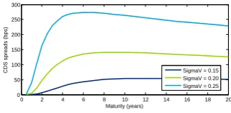
4 Modeling 31 4.1 Model 1: Constant default barrier . . . 31
4.1.1 Model assumptions . . . 31
4.1.2 Modeling framework . . . 33
4.1.3 Parameters and Monte Carlo settings . . . 37
4.1.4 Results of model 1 . . . 38
4.1.5 Conclusions model 1 . . . 42
4.2 Model 2: Stationary leverage ratio . . . 42
4.2.1 Model assumptions . . . 43
4.2.2 Modeling framework . . . 43
4.2.3 Parameters and Monte Carlo settings . . . 45
4.2.4 Results of model 2 . . . 45
4.2.5 Conclusions model 2 . . . 48
4.3 Overview and conclusions . . . 48
5 Parameter estimation and application 51 5.1 Two applications of structural models . . . 51
5.1.1 Moody’s KMV distance to default model . . . 51
5.1.2 CreditGrades model . . . 52
5.2 Case studies: data and methodology . . . 52
5.2.1 Data . . . 52
5.2.2 Methodology . . . 53
5.3 Case studies: results . . . 54
5.3.1 Ahold . . . 54
5.3.2 AkzoNobel . . . 56
5.3.3 Aegon . . . 58
5.4 Summary and conclusions . . . 60
6 Conclusions and future research 61 6.1 Conclusions . . . 61
6.2 Future research directions . . . 62
Bibliography 63 A Appendix to chapter 3 67 A.1 Credit spread in the Merton model . . . 67
A.2 Merton model algorithm . . . 68
B Appendix to chapter 4 69 B.1 Deriving equation 4.3 . . . 69
B.2 Uniform sampling . . . 69
B.3 Monte Carlo settings Model 1 . . . 71
B.3.1 Model 1: Approach 1A . . . 71
B.3.2 Model 1: Approach 1B . . . 72
B.3.3 Model 1: Approach 1C . . . 72
B.4 Monte Carlo settings Model 2 . . . 73
B.4.1 Model 2: Approach 2A . . . 73
B.4.2 Model 2: Approach 2B . . . 74
Chapter 1
Research Design
Credit risk1 has received new and increased attention since the credit crisis. Credit risk appeared to be not just the traditional risk that financial institutions avoid when lending money, but it had become a financial instrument traded around the world.
Many new, exotic credit risk related products were developed by financial institutions and all investors seemed to want a share in it. The dramatic growth of the credit market in the past years illustrates this. For example the market for CDSs almost doubled each year since 2001 to a peak notional outstanding amount of 62 trillion US Dollars in 2007 (ISDA).
Typical examples of firms that took large positions in the new credit instruments and lend too much subprime mortgages are Bear Stearns, Lehman Brothers, AIG, Fannie Mae and Freddie Mac. In the credit crisis we saw the consequences of the high credit risk in their exposures: large capital injections of governments were necessary for the firms to survive or they ended up in bankruptcy.
It is therefore not a surprise that modeling of credit risk has again gained the interest of financial institutions, regulators and academics. They try to improve the pricing methodology of financial instruments and impose new guidelines to manage credit risk exposures. Credit risk modeling is also the topic of this thesis.
1.1
Research case
This thesis is written during an internship at Deloitte Capital Markets. Deloitte Touche Tohmatsu is the brand name of independent partnerships throughout the world that collaborate to provide business services to clients. Deloitte’s core business is audit, but the firm is also active in related consulting, financial advisory, risk management and tax services.
In it’s audit activities, Deloitte supports small and medium sized enterprizes in setting up their fi-nancial statements and verifies the fifi-nancial statements of large corporates. Since the introduction of the new IFRS accounting standard these audit activities have become more complex. Especially fair value accounting2 and hedge accounting of financial derivative contracts (IAS 39) is a difficult task, and therefore specialist teams support the audit. The Deloitte Capital Markets (CM) department is one of these supporting teams.
The valuation of financial instruments is one of this teams’ specializations. The products range from plain vanilla interest rate derivatives as foreign exchange forwards and interest rate swaps, to more complex instruments as swap contracts, option-type contracts, credit derivatives and CDOs. In this thesis we focus on the valuation of CDS contracts.
Currently, the CM team applies a reduced form approach to value CDS contracts. The advantage of this approach is its speed in use. However, the method is sensitive to the selected input market data and limited in its applications.
1The terminology regarding credit risk and CDSs used in this chapter is further explained throughout chapters 2
and 3.
1.2. RESEARCH OBJECTIVES AND STRATEGY
Since the reduced form approach does not provide any additional information on variables affecting the valuation of the contract and does not allow for any credit risk analysis of a client, it is valuable for CM to develop a new credit risk model. Such a model needs to be useful for CDS valuation and should be able to provide information for other business opportunities.
1.2
Research objectives and strategy
CM’s current practice on CDS valuation and the exploration of new business opportunities related to credit risk and market risk management are the guidelines for this thesis. We define the following research objective:
Determine a credit risk model that:
1. can be used to value single name cash settled CDS contracts, 2. is able to estimate CDS term structures observed in the market, 3. can evaluate multiple credit risk measures as output,
4. and can be used to analyze the effects of market risks on these measures.
Since most CDS contracts that Deloitte CM values are single name CDSs that are settled in cash and have a maturity between 3 and 10 years, the model should be able to value at least these types of contracts. Furthermore, the model should be able to calculate CDS term structures that have sim-ilar shapes as CDS term structures observed in the market. The estimated CDS spreads should be comparable to the market CDS spreads within an acceptable range that depends on the application. The model should also be able to calculate other credit risk measures than CDS spreads, like default probabilities and recovery rates. In this way the model has more applications than CDS valuation. These measures could for example be used as inputs to the advanced credit risk modeling approach in Basel II (internal ratings based approach). Finally, it should be possible to analyze the effect of market risk, e.g. changes in interest rates and equity volatility, on the calculated credit risk measures.
To design a credit risk model with these objectives we perform our research in three phases: a literature study, a numerical analysis, and an empirical study. Each of these phases has its own goals:
Literature study. The literature study will give us more insight on (a) credit risk and its modeling approaches and (b) credit default swaps and its pricing methods. From this information we deter-mine the type of credit risk model that can be used for the valuation of CDS contracts and is able to perform a sensitivity analysis to additional credit risk measures.
We find that the structural credit risk models can meet the objectives of this study. Literature on these models is further reviewed to specify the structural models that are implemented in the numer-ical study.
Numerical analysis. Two selected models from the literature review are further analyzed in a numerical study. We focus on modeling CDS term structures and therefore implement different simu-lation algorithms in Matlab. To investigate the opportunities of the models, we perform a sensitivity analysis in which we study the effect of changes in the values of input parameters to modeled CDS term structures.
Empirical study. In this last phase we test the practical application of the selected models. We perform case studies in which we estimate the input parameters for the models from the market and balance sheet data of Dutch firms. With these input parameters we estimate the firm’s market CDS spread to test the performance of our models and identify difficulties when the models are used in practice.
1.3
Outline
Chapter 2
Credit risk and credit default swaps
This chapter introduces credit risk and credit default swaps (CDSs) from a modeling perspective. First, we explain credit risk and credit risk measurement. Then we describe various credit risk models identified in the literature and make a comparison to select the type of credit risk model that best meets the research objectives.
The chapter continuous with an introduction to credit derivatives and further focusses on CDSs. The basics of the CDS are explained and the most important aspects of CDS contracts are specified. Various methods for pricing CDS contracts are briefly discussed and a discounted cash flow method is derived in detail. Finally, we review empirical literature to identify the factors that affect CDS spreads in the marketplace. In this chapter we follow Duffie & Singleton (2003), Hull (2006) and Sch¨onbucher (2003).
2.1
Credit risk
An investor that enters into a financial transactions is faced to various risks. Two important risk types are market risk and credit risk. Market risk is the risk of value changes in a financial asset due to changes in market variables, e.g. interest rates, exchange rates, equity prices, and commodity prices. Credit risk and its measurement are explained below.
2.1.1
Explanation of credit risk
Credit risk can be defined as the risk of a loss due to the inability of a counterparty in a financial contract to fulfill its obligations.
This definition identifies several components associated with credit risk. A simple example of a financial transaction illustrates these items: a bank provides a loan of EUR 1m to a firm and they agree that the firm repays the loan one year from now.
The bank lends the money to the counterparty in the contract, the firm. From this moment, the bank faces the credit risk of the transaction. Usually, the firm repays the outstanding amount of EUR 1m (and interest) to the bank. However, if the firm gets into financial distress and eventually defaults the firm cannot repay the loan.
If such a credit event occurs, a procedure is started to recover funds from the firm’s assets to (partially) repay the bank and other lenders. This probably results in a large loss to the bank: for example only 40% of the loan might be recovered resulting in a loss of EUR 0.6m.
The example illustrates that credit risk in a financial transaction can result in large losses. Therefore, lenders will carefully assess this risk of a counterparty before they enter into the contract.
2.2. CREDIT RISK MODELING
2.1.2
Credit risk measurement
Since losses due to credit risk can be high, regulatory institutions force investors, especially financial institutions, to actively model and measure the credit risk in their portfolio. Credit risk modeling is discussed in section 2.2. This section describes the measurement of credit risk.
The Basel II framework on capital requirements for credit risk identifies the following most widely used parameters associated with credit risk measurement:
• Exposure at default (EAD).The EAD measures the extend to which an investor is exposed to the counterparty in case of a default event at the counterparty. The EAD is the outstanding amount of the contract at default and thus the maximum amount that could be lost. The EAD in the example above is EUR 5m.
• Loss given default (LGD).This is the percentage of the EAD that is lost on a contract when the counterparty defaults. One minus the LGD gives the recovery rateRRof an asset. This is the assets value recovered when a default event occurs. In the example, the LGD 60% andRR is 40%.
• Probability of default (PD). This is the probability that a default event occurs at the counterparty of a financial contract in a given time period.
• Effective maturity. The effective maturity of a financial contract is the longest possible period available to the counterparty to fulfil all of its contractual obligations. In the example, the effective maturity is one year.
Next to CDS spreads, the model that we determine in this study should be able to calculate these credit risk measures. The next section gives an overview of credit risk models that can at least model the PD.
2.2
Credit risk modeling
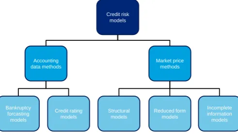
Credit risk can be modeled with different approaches. The literature distinguishes between methods that use (historical) accounting information to asses or forecast the credit risk of a firm, and methods that use market prices of assets to model credit risk. Figure 2.1 shows a further classification of the models.
© 2009 Deloitte Touche Tohmatsu
1 Footer
Credit risk models
Accounting data methods
Market price methods
Bankruptcy forcasting models
Credit rating models
Structural models
Reduced form models
Incomplete information
[image:20.595.173.419.459.598.2]models
Figure 2.1: Classification of credit risk models.
The models are developed through time to adjust for new market conditions, improve performance and to find new applications. For example Basel II’s standardized approach for calculating capital requirements for credit risk uses credit ratings, and Moody’s KMV distance to default model uses the structural model framework. The following sections shortly introduce the credit risk models in figure 2.1, such that we can make a comparison.
2.2.1
Bankruptcy forecasting models
and changes in financial ratios of firm’s that ended up in bankruptcy to design the following model:
Z = 0.012X1+ 0.014X2+ 0.033X3+ 0.006X4+ 0.999X5
where X1 = Working capital/Total assets
X1 = Retained earnings/Total assets
X1 = Earnings before interest and taxes/Total assets
X1 = Market value equity/Book value equity
X1 = Sales/Total assets
Z = Overall index.
Firms with a Z-score higher than 2.99 are considered healthy and thereby not likely to enter into bankruptcy. Firms with a Z-score lower than 1.81 are bankrupt. Firms with scores between 1.81 and 2.99 are in the so called ‘grey area’, meaning that their future is uncertain.
Altman (1968) shows that the model is accurate in forecasting bankruptcy up to two years between the bankruptcy event. Since 1968, the Z-score model is updated by Altman and other researchers to account for recent market trends by adjusting the model’s parameters and ratios.
2.2.2
Credit rating models
Credit rating models summarize credit risk in a credit rating. A credit rating is an opinion about the future credit risk of a firm. Credit rating agencies assign a credit rating to an issuer of debt based on their opinion on the ability and willingness of the issuer to meet its financial obligations. Each credit rating agency uses its own methodology to estimate this credit worthiness of the issuer based on available information on the issuers financial conditions.
The three main credit rating agencies are Standard & Poor’s, Moody’s and Fitch1. Table 2.1 shows the ratings they assign to long-term obligations2 and their meaning. Standard & Poor’s and Fitch
Table 2.1: Credit ratings of long-term obligations and their meaning. AAA to BBB rated obligations are called investment grade. Lower rated obligations are speculative grade.
Standard & Poor’s Moody’s Meaning Fitch
AAA Aaa Highest credit quality, minimal credit risk
AA Aa Very high quality
A A High quality
BBB Baa Good quality, adequate payment capacity
BB Ba Speculative, long-term uncertainty
B B Speculative, very vulnerable to adverse business
CCC Caa High current credit risk
CC Ca Currently near default, very high credit risk
C Very near default (inevitable)
D C Default
make a further classification within the categories AA to CCC by the addition of a (+) and (–) sign. Moody’s makes this relative classification within the Aa to Caa categories by adding 1, 2, or 3. A (+) and a 1 indicate that the obligation is ranked in the higher end of its class, and a (-) or 3 refers to the lower end of its category.
Credit ratings can apply to firms or countries, and to individual debt issues. When different assets have the same rating, this does not mean that the credit risk of these assets is the same. A credit rating gives an indication of the credit risk of an asset relative to the credit risk of other assets within its class.
Credit ratings can be used to determine a firm’s PD. Rating agencies provide probabilities that a
1Ratings are not only assigned by commercial rating agencies. Many financial institutions have their own internally
developed methodologies, used in for example the internal ratings based approach for their Basel II compliancy for credit risk.
2.2. CREDIT RISK MODELING
firm with a certain rating defaults within a certain time periods. Consider for example figure 2.2 that shows the average cumulative default rates for various credit ratings determined by Moody’s.
0 2 4 6 8 10 12 14 16 18 20
0 20 40 60 80 100
Term (years)
Average cumulative default rates (%)
[image:22.595.121.449.116.272.2]Aaa Aa A Baa Ba B Caa
Figure 2.2: Cumulative default rates for various credit ratings over the period 1983-2008 (Moodys Investors Service 2009).
Observe that the default rates largely differ across ratings: the higher the rating, the lower the PD. For investment grade bonds, the PD increases with time. This is because a high rated firm is considered healthy in its first years, but when time passes the probability of a change in its financial conditions increases and thus the PD increases. For lower rated firms the PD strongly increases in its first years, but the marginal PD declines when time passes. Hull (2006) explains that when a firm that is initially considered unhealthy survives its first critical years, the firm is likely to have improved its financial condition, such that the marginal PD declines.
Another observation from figure 2.2 is that default rates are positive even for short maturities. Only AAA-rated firms have PDs of approximately zero over a short horizon. This implies that firms do default on short term debt issues. Chapter 3 further elaborates on these observations.
Credit rating agencies also provide transition matrices that give the credit migration risks of firms. This is the probability that a firm with a certain rating gets an upgrade or downgrade in rating within a certain time period.
Credit ratings are an easily accessible source of information about a firm’s credit risk. However, credit ratings do not provide an up-to-date indication of credit risk, since they are not frequently updated. In the recent credit crisis we saw the consequences of this: the sudden changes in financial conditions of firms were not yet reflected in the firm’s credit rating. Firms that used credit ratings as the only source of credit risk information were thereby unable to make a correct assessment of their counterparty’s credit risk and incurred high losses.
2.2.3
Market price methods
Reduced form models, or intensity models, are developed to take the sudden nature of default events into account. There are several approaches within the reduced form models to determine default probabilities. Central in these models is the default intensity obtained from market prices of default-able instruments, such as bonds and CDSs. This default intensity is used in an exogenous arrival or jump process to model the default event. Deloitte CM uses a reduced form model to price CDS contracts in which PDs are often determined from market prices of bonds.
Reduced form models are computationally fast. However, since they do not use information from the firm’s balance sheet, they provide little economic interpretation for the default event and are not able to provide additional credit risk measures next to the PD.
Incomplete information models try to combine the properties of structural and reduced form models (Elizalde (2005c)). The structural models are used to account for the economic interpretation of the default event, and the reduced form approach has to account for the unexpected nature of default. In these models, as in the structural approach, a firm defaults when the asset value is too low to serve the obligated payments (the default threshold). However, by assuming that investors do not have complete information on the firm’s assets value and default threshold, the default event happens unexpectedly3 as in the reduced form approach.
2.2.4
Comparison of models
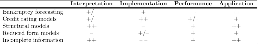
The credit risk models described in the previous sections have both advantages and disadvantages. To determine which types of models are best able to meet the research objectives, we compare them across the following dimensions4:
• Interpretation. This dimension reflects whether the credit risk model provides an economic interpretation for the occurrence of a credit event and is able to analyze this event in changing market conditions.
• Implementation. Implementation concerns the ease of obtaining the credit risk information from the model. This comprises data requirements (availability and amount), parameter esti-mation procedures, and complexity of the model.
• Performance. This indicates whether the credit risk information provided by the model is up-to-date and whether estimate measures of credit risk are comparable to market measures.
• Application. This refers to the scope of applications of the models, such as the estimation of several credit risk measures, pricing of securities and ability for market risk analysis.
[image:23.595.81.514.455.530.2]The models are compared from the perspective of a lender that wants to assess the credit risk of its counterparty in a financial contract. Table 2.2 compares the models by assigning a relative score to each of the models on every dimensions. A (++) refers to the relative highest score and (– –) to the lowest.
Table 2.2: Comparison of credit risk models.
Interpretation Implementation Performance Application
Bankruptcy forecasting +/– + – –
Credit rating models +/– ++ +/– +
Structural models ++ – + ++
Reduced form models – +/– + +
Incomplete information ++ – – + ++
The bankruptcy forecasting models are easy to implement when the financial data is available. How-ever, the model’s parameters and ratios do not always reflect the current economic conditions. Fur-thermore, these models only forecast bankruptcy and are not able to provide other output.
The advantages of credit ratings are that they are easily available for many asset classes. However, rating agencies mainly provide ratings for large, listed companies and these ratings are not frequently updated.
Structural models provide an economic explanation for the default of a firm, and as we will see in chapter 3 structural models can be designed to estimate several credit risk measures and to calculate prices of bonds, equity and CDS spreads. Major drawback of structural models is parameter estima-tion of assets value process.
The reduced form models can be used to asses the credit risk of various asset classes of firms with available market data. Implementation of reduced form models takes less effort than structural mod-els, but they do not provide an explanation for the default event and cannot provide additional output.
3See section 3.2 for more details on the expectable nature of the default event in structural models.
2.3. CREDIT DERIVATIVES
Since the incomplete information models are a combination of the structural and reduced form ap-proach, it takes the advantages of both approaches, but the implementation difficulties rise.
From this comparison we conclude that the structural credit risk models are best able to meet the objectives of this thesis. These models can be designed to determine several credit risk mea-sures, to value single name cash settled CDS contracts and estimate market CDS term structures. Furthermore, the structural modeling approach allows for extensive analysis of the firm’s default event.
2.3
Credit derivatives
Credit derivatives are securities with a payoff depending on the credit risk of a reference entity, i.e. one or more financial instruments of firms or countries. An investor exposed to the credit risk of such a reference entity, the protection buyer, enters into a credit derivative contract to (partially) transfer the credit risk to another investor, the protection seller.
The amount of credit risk transferred and the payoff of the contract depend on the type of credit derivative. According to their payoff, we can distinguish between the following credit derivatives (Bielecki & Rutkowski (2001))5:
• Credit event instruments. These are contracts in which the payoffs are conditional on a credit event at the reference entity. Examples of these type of credit derivatives are CDSs, CDS forwards and options, credit linked notes and first-to-default baskets.
• Spread instruments. In these contracts the payoffs depend on changes in the credit quality of the reference entity (e.g. changes in the credit rating or credit spread). Examples are credit spread swaps and credit spread options.
• Total return instruments. These securities transfer both the credit risk and market risk of an asset from the protection buyer to the protection seller. Examples of this type are the total return swap and loan swap.
Next section focusses on a popular type of credit derivative: the CDS.
2.4
Credit default swaps
This section introduces CDSs. First, we give a general overview of CDSs. This is followed by an explanation of the terminology associated with CDSs from the elements of a typical CDS contract. The section ends with a description of the relationship between CDS spreads and bond yields.
2.4.1
Overview of a CDS
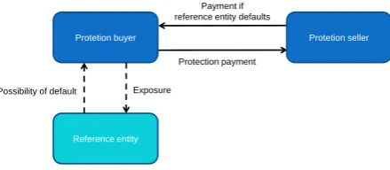
A CDS is a contractual agreement to transfer the credit risk on one or more reference entities from the buyer of the CDS contract to the seller, see figure 2.3.
Protetion buyer Protetion seller
Reference entity
Payment if reference entity defaults
Protection payment
[image:24.595.172.392.580.676.2]Exposure Possibility of default
Figure 2.3: Schematic representation of a CDS.
The protection buyer has an exposure to one or more assets of a reference entity. He takes a long
position in a CDS contract to protect for a loss in case of default of the reference entity. Another investor, the protection seller, takes a short position in this contract and agrees to compensate for this loss when such a credit event occurs. In exchange for the protection the buyer of the contract pays a premium to the protection seller, the CDS spread.
In the standard CDS contracts this premium is a periodic payment until default or maturity of the contract, whichever comes first. This type of contract is also called a running CDS, since the protec-tion payments run throughout the life of the contract. Another type of contract considers an up-front premium. In these contracts the protection buyers pay only an up-front payment at initiation of the contract in return for protection until maturity.
CDSs are traded in the over-the-counter market and can be written on single-name reference entities, indices and tranches of structured credit products. The contracts are quoted on reference entities in the market with a CDS spread and recovery rate. Bid quotes refers to the protection buyer and an offer quote to the protection seller. We study CDS contracts in more detail in the next section. According to the International Swaps and Derivatives Association (ISDA) CDSs strengthen the fi-nancial system, because:
• Banks can use CDSs to transfer credit risk to other investors, such that they can provide more debt to the market.
• CDSs distribute credit risk throughout the financial market to prevent for credit risk concen-tration.
• CDSs can be used to extract timely information on the credit quality of firms and therefore help in supervisory activities.
However, the recent credit crisis showed that there are also many risk associated with CDS contracts. First, the valuation of CDSs and other more complex credit derivatives requires understanding of advanced financial models, which make the pricing of products less transparent. Second, the CDS market is highly unregulated. For example this made it possible for AIG to trade a huge number of CDS contracts resulting in large off-balance sheet exposures towards credit risk. If the US government did not intervene with billions of support, AIG would have probably been defaulted in the credit crisis. And more recently, CDS investors were blamed to speculate on a default of Greece. The spread that the Greek government needs to pay for borrowing new money strongly increased, such that the country incurred payment difficulties.
Thus CDS contracts have advantages and disadvantages. Therefore regulatory bodies as the BIS and ISDA impose new requirements on CDS trading as a trade off between strengthening the financial system and the risks that CDSs may cause.
2.4.2
Elements of a CDS contract
This section introduces the information specified in CDS contracts, such that we can include this in the CDS pricing framework that we develop in section 2.5.
The majority of single name CDS contracts are specified according to the standards of the ISDA and comprise at least the following information:
• The reference entity. The buyer of the contract has an exposure to the reference entity (e.g. a firm) and agrees with the CDS contract to transfer the credit risk of this reference entity to the protection seller.
• The reference asset. The assets of the reference entity for which the protection buyer wants to transfer the credit risk. There is no requirement that the protection buyer owns the reference asset. Then the CDS contract is used for speculation.
• The credit event. The CDS contract is initiated to protect the buyer of the contract for a credit event at the reference entity. The CDS contracts specifies which events trigger the default payment of the protection seller to the buyer. The default events for CDSs are specified by the ISDA6:
– Failure to pay
– Bankruptcy, filing for protection
2.4. CREDIT DEFAULT SWAPS
– Restructuring (e.g. coupon reduction or maturity extension) – Repudiation/moratorium
– Obligation acceleration, obligation default (e.g. violations of bond covenants)
• The notional value of the CDS.This is the value of the reference assets that is protected by the contract.
• The starting date of the CDS.The date at which the default protection starts.
• The maturity date. The end date of the contract conditional on no credit event.
• The CDS spread. The CDS spread is the price for the default protection, measured in basis points7of the notional value. Multiplication of the CDS spread with the notional value and day count convention, gives the periodic premium payment of the protection buyer to the protection seller.
• Frequency and day count convention for premium payments. The contract specifies the period between successive premium payments, typically quarterly or semi-annually. The first payment is usually made at the end of the first period. When a credit event occurs between two payment dates, the protection buyer needs to make a final accrual payment to the protection seller. This is the payment for the protection between the last payment date and default date. The usual day count convention for CDSs is actual/360.
• Settlement terms at a credit event. If a credit event occurs before maturity, a CDS contract can be settled either physically or in cash. In a physical settlement, the protection seller buys the reference assets from the protection buyer for their notional value in exchange for the defaulted asset. In a cash settlement, the protection seller pays the difference between the notional value and the post-default market value8 of the assets to the protection buyer.
Most CDS contracts that Deloitte CM values are single name contracts with a financial institution as reference entity, settlement in cash and with maturities between 3 and 10 years. Before we develop the pricing framework for these type of CDS contracts, we first elaborate on the relation between CDS spreads and bond yields that is used in the structural model framework.
2.4.3
CDS spreads and bond yield
The CDS spread that we described in the last section is an example of a credit spread. In general a credit spread is the premium that an investor requires as a compensation for the credit risk of a financial instrument. The larger the credit risk of an investment, the larger the credit spread an investor demands.
The credit spread is measured as the difference in returns between a risky investment and an equivalent risk-free investment. For example the credit spread is the difference between the return on a corporate bond (the bond yield), and the return of a similar risk-free bond. Also, the credit spread is equal to the CDS spread, since the CDS spread is the compensation for transforming a risky investment into a risk-free investment.
From these observations we infer the following relationship between the CDS spread, c, the bond yield, y, and the risk-free rate, r, of investments with the same maturity and notional value of the (underlying) bond: c=y−r. This relationship should hold, otherwise an investor can arbitrage to lock in an immediate profit9.
However, Hull et al. (2004) impose numerous restrictions on this relation. The choice of the risk-free interest rate is an important point of interest. Bond traders often use Treasury zero curves for the risk-free rate and they measure the corporate bond yield spread as the spread of the corporate bond yield over similar treasury bonds. In this way it is assumed that the yield only reflects the credit risk of the corporate bond.
As we will see in section 2.6 however, there are many other factors that affect the yield on a bond, e.g. liquidity, such that this measure of the yield spread is incorrect. An alternative for the risk-free
7One basis point (bps) is 0.01%.
8The post-default market value of the reference assets depends on broker quotes from which the recovery rate is
determined.
rate is the LIBOR/swap rate often used by derivative traders. This rate is not totally risk-free and therefore captures some of the deficiencies of the Treasury zero rates.
CDS spreads are assumed to be a purer measure of credit risk (see also section 2.6) and thereby less affected by other factors than credit risk. We will use the Euro/swap curve for the risk-free interest rate in our modeling framework and leave the effects of liquidity and other variables for future research.
2.5
CDS valuation
This section develops the framework for valuing CDS contracts. We first give a short introduction to the hedge-based and bond yield-based pricing methods. Then we describe in more detail the discounted cash flow method that will be applied to our credit risk model.
2.5.1
Hedge-based valuation
The main points in hedge-based pricing of CDS contracts are (Sch¨onbucher (2003)):
• The method is based on the assumption that contracts with exactly the same cash flows occur-ring at exactly the same time should have the same price, otherwise an arbitrage opportunity exists.
• The price of a CDS can thus be determined from constructing and pricing a portfolio of assets with exactly the same payoff.
• The method is popular because it provides hedge strategies and does not require complex pricing models.
• Results of the method are often imprecise and it cannot be used when prices of the required assets for the replication portfolio are not available.
2.5.2
Bond yield-based pricing
In the bond yield-based pricing methods we identify the following main points (Hull et al. (2000a)):
• This method assumes that the market’s assessment of a firm’s credit risk is reflected in the difference in market price (or yield) of a defaultable bond and a risk-free bonds with the same payoffs and maturity.
• From the comparison of these securities, the probability of default of the issuer of the defaultable bond can be derived. This comparison method is also used in the reduced form modeling approach.
• Next the price of the CDS is calculated with the discounted cash flow method method described in the next section.
• A main concern in this approach is the choice of the risk-free interest rate and the impact of other non-credit risk factors on the yield spread of defaultable bonds, see also sections 2.4.3 and 2.6.
2.5.3
Discounted cash flow method
2.5. CDS VALUATION
Assumptions and terminology
The framework is developed to value single name, cash settled CDS contracts of various maturities to meet the research objectives. We make the following assumptions for this framework:
• The recovery rate used in the framework is the recovery rate on which the CDS is quoted.
• There is no correlation between the risk-free interest rate and credit risk.
• Only default of the reference entity is considered, counterparty credit risk is ignored.
• The CDS spread specified in the contract is constant and upfront spread payments are not allowed.
The value of the CDS is evaluated using risk-neutral valuation. This means that the present value of the CDS is equal to the expected value of its future cash flows discounted at the risk-free rate. By applying risk-neutral valuation we assume that the market price of risk is zero and therefore we work under the risk-neutral or Qprobability measure. Expectations under this Q-measure are expressed as EQ.
The pricing formulas will be derived for a CDS contract that is initiated a timet0= 0 with maturity T. The protection buyer makes periodic payments at daystp with p= 1,2, . . . , z until maturity or
default at time τ∗, whichever comes first. The number of default payments isz. Conditional on no default, the maximum number of protection payments is z = T /∆t, where ∆t is the time period between successive payments, ∆t = ti−ti−1, is specified in the contract. Each periodic payment
provides protection against default of the reference entity for the period [ti−1, ti].
Survival probability
The survival probability is used to determine the expected cash flows of the CDS contract. Until maturity or default of the contract, the reference entity survives and the protection buyer makes periodic payments to the seller. When a default event occurs the protection payments stop and the protection seller makes a default payment to the buyer.
Since we apply the risk-neutral valuation framework, expected losses from default are discounted at the free interest rate. This is a valid procedure if the expected losses are calculated in a risk-neutral world and this implies that PDs in this valuation framework are risk-risk-neutral.
Default probabilities determined from historical data are real-world PDs. Differences between the risk-neutral and real-world PD are explained from the excess return on defaultable bonds. According to Hull (2006) this excess return could have different reasons, as for example illiquidity and default correlation of defaultable bonds. When there is no excess return the risk-neutral and real-world PD would be the same.
The distribution of the firm’s risk-neutral probability of default qt is determined with the
struc-tural model. Integration ofqtgives the cumulative probability of defaultQt. Then, the risk-neutral
probability that the firm will not default until time tis
St= 1−Qt= 1−
Z T
0 qtdt.
We use this survival probability to define an indicator functionI(t):
1{τ∗>t}=
1 ifτ∗> t 0 ifτ∗≤t
The indicator function has a value of one with probabilityS(t) conditional of no default event up to time t. If a default event occurs at time τ∗, the indicator function has a value of zero. We use the indicator in the pricing formulas for the CDS that we introduce in the next section10.
10In general
1xyz=
Pricing formulas
The value of a CDS contract equals the present value of the expected cash flows from the contract. Below, we first determine the present value of the cash flows from the protection buyer and protection seller. With these expressions we then construct the pricing formula for the CDS.
The present value of the cash flows from the protection buyer to the seller consists of two parts:
• The expected present value of the periodic payments until maturity or default. If a credit event occurs before time ti, the ith and following payments are not paid. The premium payment at
timetiisN c0,T∆ti1{τ∗>t}, wherec0,T is the par CDS spread of a CDS contract issued at time t0= 0 with maturityT.
• The expected present value of the accrual payment that needs to be paid by the protection buyer when a default event occurs between two payment dates. This accrual payment is N c0,T(τ∗−
ti−1).
From this the expected present value of the total payment made by the protection buyer equals:
EQ " z
X
i=1
N c0,T∆tie−rti1{τ∗>t
i}+N c0,T(τ
∗−t
i−1)e−rτ
∗
1{ti−1<τ∗<ti}
#
. (2.1)
If the reference entity defaults at time τ∗, the protection seller makes a default payment to the protection buyer. We assumed that this settlement is made in cash, such that the default payment equals the expected present value of the LGD of the contract and is written as
EQhN(1−R)e−rτ∗
1{τ∗≤T} i
. (2.2)
Now the market value of a long position in a CDS is the present value of the expected default payment (2.2) minus the present value of the expected premium payments (2.1):
EQhN(1−R)e−rτ∗1
{τ∗≤T}
i − EQ " z X i=1
N c0,T∆tie−rti1{τ∗>t
i}+N c0,T(τ
∗−t
i−1)e−rτ
∗
1{ti−1<τ∗<ti}
#
.
(2.3)
A CDS contract is constructed such that the value of the contract is zero at initiation. This is done by specifying a CDS spread that equates the the present value of the protection and default payments. Setting equation 2.3 equal to zero and solving for the credit spread yields:
c0,T =
EQ
N(1−R)e−rτ∗1
{τ∗≤T}
EQPz
i=1 N∆tie−rti1{τ∗>t
i}+N(τ
∗−t
i−1)e−rτ
∗
1{ti−1<τ∗<ti}
. (2.4)
Equation 2.4 gives the par CDS spread of a CDS contract issued at timet0= 0 with maturityT. The expression in equation 2.3 can be used to determine the value of a single name, cash settled CDS contract when the default timeτ∗ is determined with a credit risk model. However, in the following
chapters of this study we focus on the calculation of CDS spreads with equation 2.411. We evaluate this expression for various maturities to obtain a CDS term structure. Modeled CDS term structures are further analyzed in chapter 4.
2.6
Credit spread puzzle
Equation 2.4 shows that CDS spreads depends on the survival probability and thus the credit risk of the reference entity. However, market CDS spreads are often found to be higher than the spreads obtained from credit risk models. This implies that credit risk is not the only factor that determines market spreads.
2.6. CREDIT SPREAD PUZZLE
This section gives an overview of empirical studies that analyze this ‘credit spread puzzle’12. In this overview we first present the main findings of studies that analyze bond yield spreads, since this market exists longer than the CDS market, and then the main findings on CDS spreads. We identify determinants besides credit risk that affect the credit spread, such that we could account for these factors in the development of the structural models in chapter 4.
2.6.1
Bond spreads
Collin-Dufresne, Goldstein, and Martin (2001) (CGM) analyze market spreads of corporate bonds. They test whether the following factors affect spread changes:
• Changes in the risk-free interest rate. A higher risk-neutral interest rate, reduces the credit spread.
• Changes in the slope of the yield curve. An increase in the Treasury yield curve13, increases the expected interest rate, and thus reduces the credit spread.
• Changes in leverage14. An increase in the firm’s leverage, increases the credit spread.
• Changes in volatility. Intuitively, when volatility increases, the probability of default in-creases.
• Changes in the probability or magnitude of a downward jump in firm value. In section 3.3.4 we will see that this increases the credit spread.
• Changes in the business climate. A better business climate15lowers the credit spread. CGM find that these factors explain approximately a quarter of the variation in the market spreads. The remaining variation could be explained by a single unidentified factor, which CGM describe as a result of supply and demand shocks.
Campbell & Taksler (2003) conduct a similar analysis as CGM and conclude that firm specific equity volatility is an important determinant of the corporate bond spread.
Cremers et al. (2006) find that option implied volatility could account for almost one third of the total variation in credit spreads. Furthermore they show that a structural model is able to explain the variation in credit spreads and that there is no evidence of a large unidentified factor affecting spreads as reported by CGM.
Huang & Huang (2003) conduct an empirical analysis of the credit spreads modeled by various structural models. They find that credit risk accounts for only a small fraction (20-30%) of the observed corporate spread for investment grade bonds of all maturities. For junk bonds, however, credit risk accounts for a much larger fraction.
2.6.2
CDS spreads
Skinner & Townend (2002) are the first to analyze the difference between model and market CDS spreads. They claim that CDS can be viewed as a put options. Therefore they analyze whether vari-ables that impact option pricing also impact CDS spreads. They show that the risk-neutral interest rate, the yield of the underlying asset, the maturity and the volatility, are also important in pricing credit default swaps.
Ericsson et al. (2005) conduct a similar research as CGM on CDS spreads. They show that the leverage of the firm, the volatility of the firm’s assets and the risk-neutral interest rate explain ap-proximately 60% of the market CDS spread. They also asses the impact of changes in these variable to changes in the CDS spread. They find that a 1% increase in annual equity volatility increases the CDS spread by 1 to 2bps and that a 1% change in the leverage of the firm raises the CDS spread by approximately 5 to 10bps. Furthermore Ericsson et al. find only weak evidence for a common unidentified factor as CGM describe.
12The presented empirical literature uses the term ‘credit spread puzzle’ for the observation that credit spreads are too high to be explained by only credit risk.
13The Treasury yield curve describes the relation between the interest rate on a Treasury bond (assumed to be
risk-free) and its time to maturity.
14CGM define leverage as the book value of debt divided by the sum of market value of equity and book value of debt.
Zhang et al. (2005) test with a structural model the impact of the firm’s equity volatility and jump risk on the credit spread. They are able to explain 77% of the variation in CDS spread by using this approach.
Alexander and Kaeck (2008) find that interest rates, stock returns and implied volatility have a signif-icant impact on CDS spreads. They again find evidence for a systemic factor as CGM. Furthermore, they show that the impact of the variables differs with the overall market conditions. They show that CDS spreads are sensitive to implied volatility in turbulent times and more sensitive to stock returns in ordinary market conditions.
Bongaerts et al. (2008) study the effects of expected liquidity and liquidity risk on CDS spreads. They find evidence for a systematic liquidity factor in the CDS market and conclude that liquidity factors need to be considered in a CDS pricing model.
Das & Hanouna (2008) observe that CDS spreads are less affected by liquidity and other non-credit risk related factors than bond spreads. However, they show via a hedge relationship between the credit and equity market that CDS spreads are negatively related to the equity liquidity of the refer-ence entity.
We emphasize that this literature review is not exhaustive, but we can observe the following:
• Credit spreads modeled with a structural framework show high correlation with market spreads. However, the modeled spreads are lower than the corresponding market spreads due to non-credit risk related factors. Bond spreads seem to be more affected by these factors than CDS spreads. This suggest that structural models are better able to estimate CDS spreads than bond spreads. This is further investigated in section 3.4.
• The literature identifies several (unidentified) factors that explain part of the credit spread besides credit risk. Most studies agree on the sign of the relations between the credit spread and factors. However, the magnitude of the impact differs amongst studies due to differences in data sets.
This study focusses on modeling CDS term structures and therefore we need to take these factors into account in our modeling approach. We will do this when we the select the components of the structural model that we will implement at the end of chapter 3. And we assess the impact of several (market risk) factors on CDS term structures in chapter 4. As stated before, liquidity factors are left for future research.
2.7
Summary
Chapter 3
Structural models
Chapter 2 determined that structural models of credit risk are best able to meet the objectives of this thesis. This chapter further investigates these models and starts with a description of the first structural model developed by Merton (1974). We compare PDs and CDS spreads evaluated with this model to market data and identify the model’s shortcomings. Then we examine extensions to the Merton model that address the Merton model’s shortcomings, and describe the implications of these extensions for credit risk modeling. Finally, we review empirical literature to assess the performance of structural models in modeling credit spreads. Based on this literature review, we select the components of the structural models that we further implement and analyze in chapters 4 and 5.
3.1
The Merton model
The literature on structural models for credit risk starts with the papers of Black & Scholes (1973) and Merton (1974). Merton develops a framework that relates the firm’s assets value to its credit risk and subsequently uses the Black & Scholes option pricing formulas to price defaultable bonds and equity of the firm.
This section describes the Merton (1974) model in more detail. We first summarize the assumptions underlying the model and analyze the conditions of default. Then we present the formulas to price equity and debt and to calculate PDs and credit spreads. The shortcomings of the Merton model are discussed in section 3.2.
3.1.1
Assumptions and default conditions
Merton (1974) makes the following assumptions to develop his model1:
1. There are no transaction costs, bankruptcy costs or taxes, such that the Modigliani-Miller theorem holds2. Assets are divisible and trading takes place continuously in time with no restrictions on short selling of all assets. Borrowing and lending is possible at the same, constant interest.
2. There are sufficient investors in the market place with comparable wealth levels, such that each investor can buy as much of an asset he wants at the market price
3. The risk-free interest rateris constant and known with certainty.
4. The evolution of the firm’s assets valueVtfollows a stochastic diffusion process:
dVt
Vt
= (µV −δ)dt+σVdWt (3.1)
1Since Merton uses the Black & Scholes (1973) methodology to price securities, Merton makes these assumptions
along with some of the Black & Scholes assumptions.
3.1. THE MERTON MODEL
whereµV is the expected return on the firm’s assets per unit time,δis the payout of the firm per
unit time3,σV is the volatility of the firms assets per unit time, anddWt is a Wiener process.
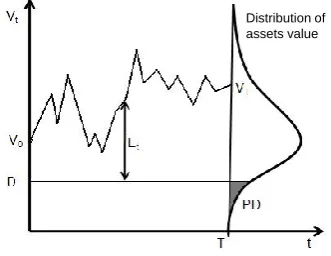
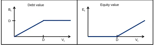
According to Merton (1974) not all of these assumptions are necessary to obtain the model, but are made for convenience. The critical assumptions are continuous time trading and assumption 4. Furthermore, the model assumes a simplified capital structure for the firm. Total debt consists of only one zero-coupon bond (ZCB) and there are no additional debt issues before maturity of the ZCB. The firm’s equity consists of ordinary shares. Both debt and equity are contingent claims on the assets of the firm and the value of total assets (or the firm value) equals the value of total debt Bt and equityEt: Vt=Bt+Et.
The ZCB has a notional amountD, which has to be paid at maturityT. When the value of the firm’s assets at maturity exceedsD, the bondholders receive the full notional amount and the shareholders receive the residual asset valueVT−D. When the asset value at maturity is less thanDthe firm
can-not make the promised debt payment and defaults. The bondholders take over the firm and receive the firm valueVT, while the shareholders receive nothing. Shareholder never have to compensate for
the bondholders’ loss in case of default, which means thatET cannot be negative.
[image:34.595.199.365.282.410.2]Distribution of assets value
Figure 3.1: Schematic representation of the Merton model, Duffie & Singleton (2003).
Figure 3.1 illustrates the dynamics in the Merton model. Observe that total debtD is constant over time and that the value of equity fluctuates with the value of the firm’s assets. Default occurs only when the firm value drops below the default barrier at maturity, such that VT < D. By simulating
various paths for the asset value process a distribution of the asset value at maturity is modeled. The shaded area of this distribution is the probability of default.
3.1.2
Security pricing and PD calculation
Based on the assumptions and default conditions described above we can derive the formulas for pricing debt and equity in the Merton framework. Since we need the Black & Scholes option pricing theory for this objective we will work under the risk-neutral probability measureQ4. We follow Hull et al. (2004) to derive the formulas.
The payoffs of debt and equity at maturity can be expressed as European options written on the firm’s assets with exercise price D and maturityT. We saw in section 3.1.1 that the payoff to the bondholders at maturity equals BT = min(VT, D). We can replicate this payoff with the following
portfolio5:
BT =VT −max(VT −D,0) (3.3)
3A positiveδis a payout to shareholders or liabilities-holders (dividends or interest respectively) and a negativeδ is the net amount received from new equity financing.
4Under this measure we set the expected return of the firms assetsµ
V equal to the risk-free interest raterto model
the firm’s asset value process (assuming zero payout, i.e. δ= 0) as a geometric Brownian motion:
dVt V t
=rdt+σdWt (3.2)
5Note that we could also replicate the debt payoff with the portfolioD−max(D−V
T,0) that is constructed from
This portfolio consists of a long position in the firm’s assets and a short position in a European call option on the firm’s assets with exercise priceD.
Once the debt has been paid at maturity the remaining assets value belongs to the shareholders. This payoff equals the payoff of a European call option written on the firm’s assets with exercise priceD:
ET = max(VT−D,0). (3.4)
The debt payoff as a function of the assets value is shown in the upper part of figure 3.2. The right graph shows the payoff to the shareholders, the payoff of a European call option.
Vt
D Bt
D
Vt
D Et
[image:35.595.165.423.180.256.2]Equity value Debt value
Figure 3.2: Equity and debt values as a function of the assets value in the Merton Model.
We can now apply the Black & Scholes option pricing formulas to determine the value of the firm’s debt and equity at timet(0≤t≤T) as
Bt=VtΦ(−d1) +De−r(T−t)Φ(d2) (3.5)
Et=VtΦ(d1)−De−r(T−t)Φ(d2) (3.6)
where Φ(·) is the cumulative standard normal distribution function andd1 andd2 are given by
d1=
ln (Vt/D) + (r+ σV2
2 )(T−t) σV
√
T−t and d2=d1−σV
√
T−t.
Figure 3.1 showed that the probability of default in the Merton model is given by the probability that the firm’s assets value is lower than the obligated debt paymentD at maturity. In the Merton framework the risk-neutral probabilityPM of default at timeT can be calculated as:
PM = Φ(−d2). (3.7)
From this equation we infer that the probability of default depends on the inverse leverage of the firm Vt/D, the volatility of the firm’s assets σV, and the time to maturity T. We further analyze these
relationships in chapter 4.
3.1.3
Credit spread in the Merton model
Finally we derive the credit spread in the Merton framework using the relationship between the credit spread, risk-free interest rate, and bond yield described in section 2.4.3: c = y−r6. The yield to maturityy of the ZCB is implicitly given by
Bt=De−y(T−t)
Solving this equation fory and then substitutingBt,T with equation 3.5 gives
yt,T =−
ln
(Vt/D)Φ(−d1) +e−r(T−t)Φ(d2)
T −t (3.8)
Now we can usec=y−rto write the CDS spread in the Merton model as
ct,T =−
ln
(Vt/D)Φ(−d1)er(T−t)+ Φ(d2)
T−t . (3.9)
The credit spread also depends on the firm’s leverage, the volatility of the firm’s assets and the time to maturity.
Equation 3.9 is specific for the Merton model. We will use equation 2.4 with an algorithm to calculate the default time to determine CDS spreads in chapter 4.
3.2. SHORTCOMINGS OF THE MERTON MODEL
3.2
Shortcomings of the Merton model
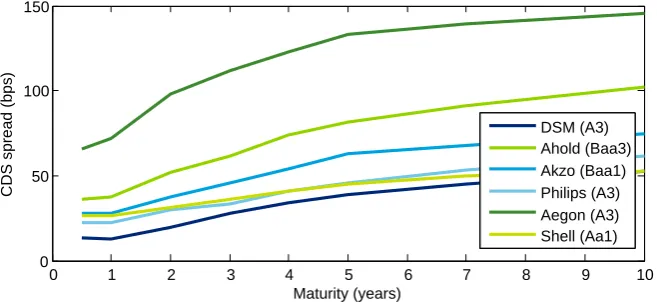
Merton’s model provides an insightful approach to assess a firm’s credit risk and to calculate debt and equity values. However, this section shows that the practical applicability of the model is re-stricted. We compare modeled PDs and CDS spreads to market data to identify the most important shortcomings of the Merton model. These shortcomings are addressed in subsequent sections. Figure 3.3 shows par CDS term structures for a number of Dutch firms with various credit ratings (Moody’s). Note that firms with a different credit rating can have approximately similar CDS spreads as for example Shell and Philips. Possible explanations are different industry risks and prospects or an ‘old’ credit rating that does not incorporate the current conditions of the firm that are already reflected in the CDS spread.
0 1 2 3 4 5 6 7 8 9 10
0 50 100 150
CDS spread (bps)
[image:36.595.122.451.225.376.2]Maturity (years) DSM (A3) Ahold (Baa3) Akzo (Baa1) Philips (A3) Aegon (A3) Shell (Aa1)
[image:36.595.99.498.479.576.2]Figure 3.3: CDS term structures of selected Dutch firms on 31-12-2009 (Bloomberg, CMAN).
Figure 3.4 plots term structures of the risk-neutral PD and CDS spread calculated with the Merton model for various levels of the promised debt payment at maturity. These term structures are ob-tained with a Monte Carlo simulation approach given in appendix A.2.
0 2 4 6 8 10 12 14 16 18 20
0 0.05 0.1 0.15 0.2 Maturity (years) Risk−neutral PD
Lev = 30% Lev = 40% Lev = 50% Lev = 60% Lev = 70%
(a)Probability of default
0 2 4 6 8 10 12 14 16 18 20
0 50 100 150 200 250 Maturity (years)
CDS spread (bps)
Lev = 30% Lev = 40% Lev = 50% Lev = 60% Lev = 70%
(b)CDS term structure
Figure 3.4: Probability of default (a) and CDS term structures (b) determined with the Merton Model for various leverage ratios. Note that this leverage ratio is defined as the ratio of the promised debt paymentD to the initial firma value. Input parameters are: r= 0.05,σV = 0.2, andV0= 100.
Over a long horizon, marginal PDs and especially CDS spreads decrease in the Merton model, while these are increasing functions in the market. This is because firms cannot issue additional debt be-tween initiation and maturity in the Merton model. Due to a positive drift in the assets value process the distance between this process and the constant promised debt payment increases such that the firm is less likely to default. Section 3.3.1 offers a solution to the model’s shortcoming of downward sloping term structures.
From the assumptions underlying the Merton model, we derive four more shortcomings. First, the debt structure of a firm is often more complicated than the Merton model assumes. Common features of a firm’s debt like coupons, covenants and embedded options cannot be modeled. In section 3.3.1 we describe structural models that allow for a more extend capital structure.
Second, in the Merton model default can only occur at the maturity of debt. This implies that a firm’s asset value can drop to almost zero and subsequently recover toD or more before maturity, without going bankrupt. In practice, such a firm would have been defaulted before default. Structural models that introduce more advanced default barriers to deal with this shortcoming are discussed in section 3.3.2
Furthermore, the Merton model assumes a constant risk-free interest rate that is known with cer-tainty. However, the term structure of interest rates observed in the market is not flat and stochastic in time. Merton makes t