An Instance of Failure for the MATLAB Explicit ODE45 Solver

An Instance of Failure for the MATLAB Explicit

ODE45

Solver

Riccardo Fazio

Abstract—We consider the adaptive strategies ap-plicable to a simple model describing the phase lock of two coupled oscillators. This model has been used to show an instance of failure of the ODE45 Runge-Kutta-Felberg solver implemented within the MAT-LAB ODE suite, see [J. D. Skufca. Analysis still mat-ters: a surprising instance of failure of Runge-Kutta-Felberg ODE solvers. SIAM Review, 46:729-737, 2004]. We compare the numerical results obtained with: the MATLAB ODE suite’s explicit solvers, and the local linearity strategy implemented with the clas-sical fourth-order Runge-Kutta method as a basic method.

Keywords: initial value problems, adaptive numerical methods, local linearity approach.

1

Introduction

We consider the adaptive strategies used for the numeri-cal integration of initial value problems (IVPs) governed by systems of ordinary differential equations

 



du

dt = f(u), t∈[t0, tmax] u(t0) =u0,

(1)

whereu(t) : IR→IRk,u0∈IRkand f(u) : IRk →IRk.

Ac-cepted strategies for variable step size selection are based mainly on the inexpensive monitoring of the local trunca-tion error, or the residual monitoring, or the definitrunca-tion of a suitable monitor function, or the utilization of scaling invariance properties. The relevant bibliography can be listed as follows.

1) Local error control, first introduced by Milne’s device in the implementation of predictor-corrector methods [11, pp. 107-109] or [9, pp. 75-81]. Extensions to embedded Runge-Kutta methods have been developed by Sarafyan [12], Fehlberg [8], Verner [18] and Dormand and Price [4].

∗_{Department of Mathematics, University of Messina,}

Con-trada Papardo, Salita Sperone 31, 98166 Messina, Italy. E-mail: [email protected] Home-page: http://mat520.unime.it/fazio

Acknowledgement. This work was supported by the Univer-sity of Messina and partially by the Italian MUR. Date of the manuscript submission: January 19, 2010.

2) Local error control based on Richardson local extrap-olation, see Shampine [15, pp. 361-364].

3) Residual (or size of the defect) monitoring, proposed by Enright [5], see also his survey paper [6].

4) Monitoring the relative change in the numerical solu-tion, proposed by Shampine and Witt [14] and recently modified by Jannelli and Fazio [10].

5) Adaptivity by scaling invariance, proposed for the nu-merical solution of blow-up problems by Budd et al. [1, 2].

We report here an application of a new strategy based on monitoring the approximate local linearity of the com-puted solution. For this strategy, preliminary numerical results, concerning the classical two body problem, were presented at the World Congress on Engineering held in London (July 1-3, 2009) [7].

2

Two coupled oscillators

Let us consider a system modeling two coupled oscillators

     dθ1

dt =ω1+k1 sin(θ2−θ1) dθ2

dt =ω2+k2 sin(θ1−θ2),

(2)

where θ1 andθ2 are the two phase angles describing the

time evolution of the two oscillators, with natural fre-quencies ω1 and ω2, respectively,k1 and k2 are the

cou-pling constants between the oscillators, andt is the time independent variable. The model (2) has been proposed and studied as a dynamicsl system [17]. As a specific test case, we will consider here the initial value problem

         dθ1

dt = 1 + sin(θ2−θ1), t∈[0, tmax] dθ2

dt = 1.5 + sin(θ1−θ2) θ1(0) = 3, θ2(0) = 0.

(3)

This problem has the exact solution:

θ1(t) =

5 4 t+

3

2 −arctan(p1)

(4)

θ2(t) =

5 4 t+

3

θ1

t θ2

θ1

t

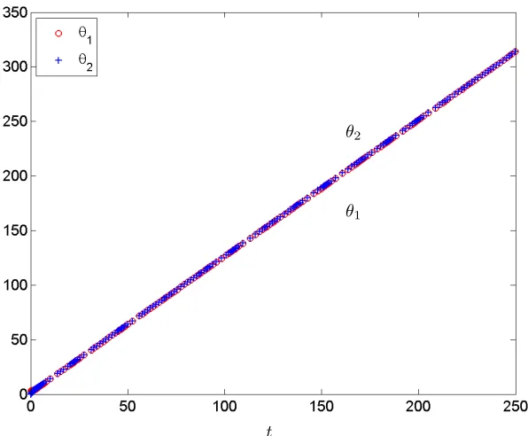
Figure 1: Numerical solution of (3) for t∈[0,250] by the MATLAB solverODE45. Left: zoom of the initial stage. Right: longer computation.

∆tn

t

Figure 2: Step-sizes used byODE45in solving (3).

where p1 = (4 p2 −15 tanh((15 t+ 4 p2 arctanh(p2 (tan(3/2) + 4)/15))p2/60))p2/15 andp2 = 15(1/2)_.

By following Skufca [16], let us try to solve problem (3) by the ODE45 solver with the accuracy and adaptivity parameters defined by default. Figure 1 shows the

nu-merical results. The two oscillators phase look by about

θ2

θ1

t θ2

θ1

t

Figure 3: Numerical solution of (3) fort∈[0,250]. Left: byODE23. Right: byODE113.

shown in figure 2 are smaller than those found by Skufca and reported on figure 2 of [16]. In particular, the adap-tivity algorithm of ODE45has been modified in order to take care of the stability limit ∆tn < 1.44 suggested by Skufca in the analysis of section 3 of his paper. So that, it is surprising to find that the decorrelation of the two oscillators is still present in figure 1. Indeed, using theodesetoption command, Skufca should have verified that by imposing ∆tmax<1.44 he would be able to

com-pute a correlated numerical solution, but he didn’t. So that, we decided to use the classical fourth order Runge-Kutta (RK4) method, see Butcher [3, p. 166], a step-size update formula similar to the one applied byODE45, and to look for a different adaptive strategy.

2.1

MATLAB explicit ODEs solvers

The numerical results given by theODE45solver have been the topic of this section. For the sake of completeness, figure 3 displays the numerical results obtained by the MATLAB explicit solvers ODE23 and ODE113. It is eas-ily seen that, for the considered problem, ODE23is more accurate thanODE113.

In the next section we describe our local linearity moni-toring.

3

Local linearity and adaptivity

This novel approach is based on the idea that, locally, every continuous solution behaves approximatively like a straight line. Therefore, a new monitor function can be

defined as follows

ϑn= 2r

1 +rj=1max,...,k

jun+1−(1 +r)jun+r jun−1 |j_un|+ (5) where r= ∆tn/∆tn−1, 0< 1, and we use the

nota-tion for the components of a vector introduced by Lam-bert [11, p. 3], so that juis the j-th component of the vectoru. Note that our monitor function (5) reduces to

ϑ∗_n= max j=1,...,k

jun+1− jun

|j_un|+ (6) when we set jun−1= jun andr= 1. Therefore, at the initial step, we can applyϑ∗n insted ofϑn only by setting the two mentioned conditions.

In order to show the meaning of our control function we recall the finite difference approximation

d2_u

dt2(tn) =

2r

1 +r

un+1−(1 +r)un+r un−1

(∆tn)2

+O(∆tn), (7) where the first two addends of the error termO(∆tn) are given by

(1−r)

r

∆tn 3

d3_u

dt3(tn) +

(r2_{−r+ 1)}

r2

(∆tn)2 12

d4_u

dt4(tn).

Therefore, our monitor function, defined by equation (5), is a first order finite difference approximation for

ϑn≈(∆tn)2 max j=1,...,k

d2 j_u

dt2 (tn) |j_u(t

n)|+

θ2

θ1

t

Figure 4: Local linearity control. Numerical solution for the problem 3.

We can also note that, if we set ∆t= ∆tn = ∆tn−1, then

the finite difference formula (7) reduces to the classical second order central approximation

d2_u

dt2(tn) =

un+1−2un+un−1

(∆t)2 +O

(∆t)2

,

where the error term O (∆t)2

has only even powers of ∆t.

4

Step size selection

As far as the adaptivity control is concerned, we can re-quire that the step size selection is such thatϑn satisfies the condition

0< ϑn≤τ ,

whereτ is a user defined tolerance bound.

As far as the control of the local error estimate is con-cerned, it has been shown by Shampine [13] that, both in the case when the step is rejected and repeated, or in the case of a successful step, the largest step size that can be used in order to get the next step a successful one, is given by

∆t= ∆tn _τ

ϑn

1/(p+1)

, (8) wherepis the order of the method used. However we are considering a different control strategy, and therefore we

are willing to apply two safe parameters, say 0< s1 <1

es2>1, for the selection of the new time step. So that,

we can use the predicted new step size

∆tn+1=  



s2∆tn if s1∆t > s2∆tn ∆tn/s2 if s1∆t <∆tn/s2

s1∆t otherwise.

(9)

In this way, we apply a reduction factor s1 of the

pre-dicted step size and, moreover, it will be true that the amplification, or reduction, factor of the previous step size never exceeds the values2.

In any case, the user have to define the following adaptive parameters: a tentative initial step size ∆t0, an upper

bound toleranceτ, a safe factors1, and a step

amplifica-tion and reducamplifica-tion factors2.

We remark that the linearity adaptive approach is based on implementing only one numerical method, and that, in order to advance the computation, it uses three numerical approximations obtained at three consecutive time steps.

5

Numerical results

Our local linearity strategy was implemented with the classical fourth-order Runge-Kutta method as a basic method. In all the simulation reported in this subsection we used the following adaptivity parameters: τ = 10−3,

∆tn

ϑn

t

Figure 5: Local linearity control. Top frame: step selection. Bottom frame: monitor functionϑn.

θ2

θ1

t

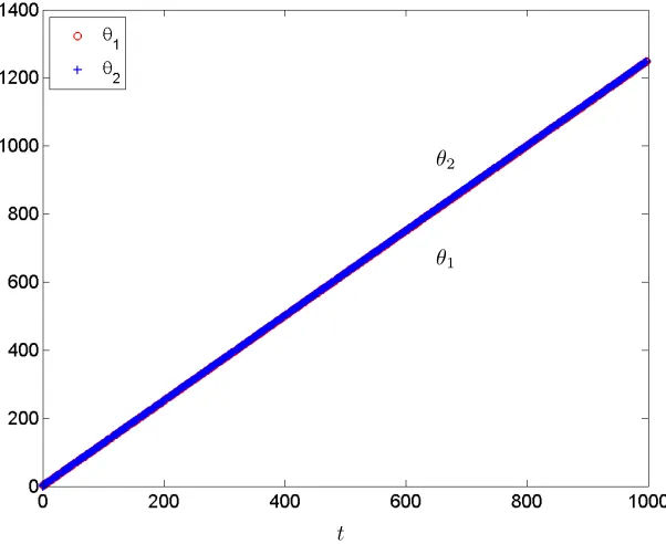
Figure 6: Local linearity control. Longer computation.

numerical results within the range t ∈ [0,250]. Our al-gorithm used 452 successful steps plus 27 rejections to compute the numerical solution. The used step sizes

were included within the limits ∆tmin≈1.21·10−8 and

∆tmax ≈4.67. Note that our ∆tmax is more than three

cerned, we used the MATLAB rounding off uniteps, that is≈2.2205·10−16_{. We had to define a tentative initial}

step, so that we used ∆t0 = 10. However, the proposed

value of the initial step size, as it is easily seen from figure (5), has been reduced by our adaptive algorithm in order to complain with the user defined tolleranceτ.

On the previous page, figure 6 shows a longer integration wheret∈[0,1000]. Let us remark here that, even for this range of the time variable, our numerical trajectories of the two oscillators do not decorrelate. Our algorithm used 894 successful steps plus 39 rejections to compute the numerical solution shown in figure 6.

6

Conclusions

It seems that, as suggested by Skufca, the crux of the

ODE45method is the step-size update formula. However, our point of view is that neither the analysis of section 3 nor the one in section 4 in Skufca paper are really valid. In fact, his argument is that being each attracting solu-tion component of the system a straight line, a Runge-Kutta method of any order should be exact in approxi-mating the slope and the error estimate has to tend to zero, so that the selected step size will increase until it becomes large enough to make the method unstable. The above reasoning has a weak point: it is only valid for step-sizes tending to zero but it makes a conclusion for large step sizes. Furthermore, it does not take into account the rounding errors of any real computation. Moreover, the same analysis can be applied to the control based on local linearity strategy, but, as we have reported in the previ-ous section, with this adaptive strategy we have obtained a correlated solution within the domaint∈[0,1000].

References

[1] C. J. Budd, B. Leimkuhler, and M. D. Piggott. Scal-ing invariance and adaptivity. Appl. Numer. Math., 39:261–288, 2001.

[2] C. J. Budd and M. D. Piggott. The geometric inte-gration of scale invariant ordinary and partial differ-ential equation. J. Comput. Appl. Math., 128:399– 422, 2001.

[3] J. C. Butcher. The Numerical Analysis of Ordi-nary Differential Equations, Runge-Kutta and Gen-eral Linear Methods. Whiley, Chichester, 1987.

[4] J. R. Dormand and P. J. Price. A family of embed-ded Runge-Kutta formulae.J. Comput. Appl. Math., 6:19–26, 1980.

ODEs with defect control. J. Comput. Appl. Math., 125:159–170, 2000.

[7] R. Fazio. Adaptive strategies for numerical IVPs solvers. In S.I. Ao, L. Gelman, D.W.L. Hukins, A. Hunter, and A.M. Korsunsky, editors,Proceedings World Congress on Engineering 2009, held in Lon-don, 1-3 July, volume II, pages 1213–1218. IAENG, Kwun Tong – Hong Kong, 2009.

[8] E. Fehlberg. Classical fifth-, sixth-, seventh- and eighth order formulas with step size control. Com-puting, 4:93–106, 1969.

[9] A. Iserles. A First Course in the Numerical Analy-sis of Differential Equations. Cambridge University Press, Cambridge, 1996.

[10] A. Jannelli and R. Fazio. Adaptive stiff solvers at low accuracy and complexity. J. Comput. Appl. Math., 191:246–258, 2006.

[11] J. D. Lambert.Numerical Methods for Ordinary Dif-ferential Systems. Wiley, Chichester, 1991.

[12] D. Sarafyan. Error estimation for Runge-Kutta methods through pseudoiterative formulas. Techn. Rep. No 14, Lousiana State Univ., New Orleans, 1966.

[13] L. F. Shampine. Error estimates and control for ODEs. J. Sci. Comput., 25:3–16, 2005.

[14] L. F. Shampine and A. Witt. A simple step size selection algorithm for ODE codes.J. Comput. Appl. Math., 58:345–354, 1995.

[15] L.F. Shampine.Numerical Solution of Ordinary Dif-ferential Equations. Chapman & Hall, New York, 1994.

[16] J. D. Skufca. Analysis still matters: a surpris-ing instance of failure of Runge-Kutta-Felberg ODE solvers. SIAM Review, 46:729–737, 2004.

[17] S. Strogatz. Nonlinear Dynamics and Chaos with Applications to Physics, Biology, Chemistry, and Engineering. Perseus Books, Cambridge, MA, 1994.