Speeding up Training with Tree Kernels for Node Relation Labeling
Jun’ichi Kazama and Kentaro Torisawa
Japan Advanced Institute of Science and Technology (JAIST) Asahidai 1-1, Nomi, Ishikawa, 923-1292 Japan
{kazama, torisawa}@jaist.ac.jp
Abstract
We present a method for speeding up the calculation of tree kernels during train-ing. The calculation of tree kernels is still heavy even with efficient dynamic pro-gramming (DP) procedures. Our method maps trees into a small feature space where the inner product, which can be cal-culated much faster, yields the same value as the tree kernel for most tree pairs. The training is sped up by using the DP pro-cedure only for the exceptional pairs. We describe an algorithm that detects such ex-ceptional pairs and converts trees into vec-tors in a feature space. We propose tree kernels on marked labeled ordered trees and show that the training of SVMs for semantic role labeling using these kernels can be sped up by a factor of several tens.
1 Introduction
Many NLP tasks such as parse selection and tag-ging can be posed as the classification of labeled ordered trees. Several tree kernels have been pro-posed for building accurate kernel-based classifiers (Collins and Duffy, 2001; Kashima and Koyanagi, 2002). They have the following form in common.
K(T1, T2) =
X
Si
W(Si)·#Si(T1)·#Si(T2), (1)
whereSiis a possible subtree,#Si(Tj)is the
num-ber of times Si is included in Tj, and W(Si) is the weight of Si. That is, tree kernels are inner products in a subtree feature space where a tree is mapped to vector V(Tj) =
³p
W(Si)#Si(Tj)
´
i. With tree kernels we can take global structures into account, while alleviating overfitting with kernel-based learning methods such as support vector ma-chines (SVMs) (Vapnik, 1995).
Previous studies (Collins and Duffy, 2001; Kashima and Koyanagi, 2002) showed that although it is difficult to explicitly calculate the inner product in Eq. (1) because we need to consider an exponen-tial number of possible subtrees, the tree kernels can be computed inO(|T1||T2|) time by using dynamic
programming (DP) procedures. However, these DP procedures are time-consuming in practice.
In this paper, we present a method for speeding up the training with tree kernels. Our target ap-plication is node relation labeling, which includes NLP tasks such as semantic role labeling (SRL) (Gildea and Jurafsky, 2002; Moschitti, 2004; Ha-cioglu et al., 2004). For this purpose, we designed kernels on marked labeled ordered trees and derived
O(|T1||T2|)procedures. However, the lengthy
train-ing due to the cost of kernel calculation prevented us from assessing the performance of these kernels and motivated us to make the training practically fast.
Our speed-up method is based on the observation that very few pairs in the training set have a great many common subtrees (we call such pairs
mali-cious pairs) and most pairs have a very small number
of common subtrees. This leads to a drastic vari-ance in kernel values, e.g., whenW(Si) = 1. We thus call this property of data unbalanced similarity. Fast calculation based on the inner product is possi-ble for non-malicious pairs since we can convert the trees into vectors in a space of a small subset of all subtrees. We can speed up the training by using the DP procedure only for the rare malicious pairs.
We developed the FREQTM algorithm, a modifi-cation of the FREQT algorithm (Asai et al., 2002), to detect the malicious pairs and efficiently convert trees into vectors by enumerating only the subtrees actually needed (feature subtrees). The experiments demonstrated that our method makes the training of SVMs for the SRL task faster by a factor of several tens, and that it enables the performance of the ker-nels to be assessed in detail.
2 Kernels for Labeled Ordered Trees The tree kernels proposed so far differ in how sub-tree inclusion is defined. For instance, Kashima and Koyanagi (2002) used the following definition.
DEFINITION2.1 S is included in T iff there exists a one-to-one functionψfrom a node ofSto a node ofT such that (i) pa(ψ(ni)) = ψ(pa(ni))(pa(ni)
returns the parent of nodeni), (ii)ψ(ni)ºψ(nj)iff
ni º nj (ni ºnj means thatni is an elder sibling
ofnj), and (iii)l(ψ(ni)) = l(ni)(l(ni)returns the
label ofni).
We refer to the tree kernel based on this definition as
Klo. Collins and Duffy (2001) used a more restric-tive definition where the preservation of CFG pro-ductions, i.e., nc(ψ(ni)) = nc(ni) if nc(ni) > 0 (nc(ni)is the number of children ofni), is required in addition to the requirements in Definition 2.1. We refer to the tree kernel based on this definition asKc. It is pointed that extremely unbalanced kernel val-ues cause overfitting. Therefore, Collins and Duffy (2001) used W(Si) = λ(# of productions inSi), and Kashima and Koyanagi (2002) used W(Si) =
λ|Si|, whereλ(0 ≤ λ ≤ 1) is a factor to alleviate
the unbalance by penalizing large subtrees.
To calculate the tree kernels efficiently, Collins and Duffy (2001) presented anO(|T1||T2|)DP
pro-cedure forKc. Kashima and Koyanagi (2002) pre-sented one forKlo. The point of these procedures is that Eq. (1) can be transformed:
K(T1, T2) =
X
n1∈T1
X
n2∈T2
C(n1, n2),
C(n1, n2)≡PSiW(Si)·#Si(T1Mn1)·#Si(T2Mn2),
where #Si(Tj M nk) is the number of times Si is
included in Tj with ψ(root(Si)) = nk. C(n1, n2)
can then be calculated recursively from those of the children ofn1andn2.
3 Kernels for Marked Labeled Ordered Trees for Node Relation Labeling 3.1 Node Relation Labeling
The node relation labeling finds relations among nodes in a tree. Figure 1 illustrates the concept of node relation labeling with the SRL task as an ex-ample. A0, A1, and AM-LOC are the semantic roles
Figure 1: Node relation labeling.
Figure 2: Semantic roles encoded by marked labeled ordered trees.
of the arguments of the verb “see (saw)”. We repre-sent an argument by the node that is the highest in the parse tree among the nodes that exactly cover the words in the argument. The node for the verb is determined similarly. For example, the node la-beled “PP” represents the AM-LOC argument “in the sky”, and the node labeled “VBD” represents the verb “see (saw)”. We assume that there is a two-node relation labeled with the semantic role (repre-sented by the arrow in the figure) between the verb node and the argument node.
3.2 Kernels on Marked Labeled Ordered Trees
We define a marked labeled ordered tree as a labeled ordered tree in which each node has a mark in ad-dition to a label. We usem(ni)to denote the mark of nodeni. If ni has no mark, m(ni) returns the special mark no-mark. We also use the function
marked(ni), which returns true iff m(ni) is not
no-mark. We can encode ak-node relation by using
kdistinct marks. Figure 2 shows how the semantic roles illustrated in Figure 1 can be encoded using marked labeled ordered trees. We used the mark *1 to represent the verb node and *2 to represent the argument node.
Algorithm 3.1: KERNELLOMARK(T1, T2)
(nodes are ordered by the post-order traversal) forn1←1to|T1|do
for8n2←1to|T2|do —————————————(A)
> > > > > > > > > > > > > > > > > > > > > > > > > > > > > > > > > > > > < > > > > > > > > > > > > > > > > > > > > > > > > > > > > > > > > > > > > :
iflm(n1)6=lm(n2)then
C(n1, n2)←0 Cr(n1, n2)←0
else ifn1andn2are leaf nodes then C(n1, n2)←λ
ifmarked(n1)andmarked(n2)then Cr(n
1, n2)←λ elseCr(n1, n2)←0
else
S(0, j)←1 S(i,0)←1
ifmarked(n1)andmarked(n2)then Sr(0, j)←1 Sr(i,0)←1
elseSr(0, j)←0 Sr(i,0)←0 fori←1tonc(n1)do
forj←1tonc(n2)do S(i, j)←
S(i−1, j) +S(i, j−1)−S(i−1, j−1) +S(i−1, j−1)·C(chi(n1), chj(n2)) Sr(i, j)←
——————————(B)
Sr(i−1, j)+Sr(i, j−1)−Sr(i−1, j−1) +Sr(i−1, j−1)·C(ch
i(n1), chj(n2)) +S(i−1, j−1)·Cr(ch
i(n1), chj(n2))
−Sr(i−1, j−1)·Cr(ch
i(n1), chj(n2)) C(n1, n2)←λ·S(nc(n1), nc(n2))
Cr(n
1, n2)←λ·Sr(nc(n1), nc(n2))
return(P|T1| n1=1
P|T
2| n2=1C
r(n 1, n2))
otherwise. To enable such classification, we need tree kernels that take into account the node marks. We thus propose mark-aware tree kernels formu-lated as follows.
K(T1, T2) =
X
Si:marked(Si)
W(Si)·#Si(T1)·#Si(T2),
wheremarked(Si)returns trueiffmarked(ni) = true for at least one node in tree Si. In these ker-nels, we requirem(ψ(ni)) = m(ni) in addition to
l(ψ(ni)) =l(ni)for subtreeSito be regarded as in-cluded in treeTj. In other words, these kernels treat
lm(ni) ≡ (l(ni), m(ni)) as the new label of node
niand sum only over subtrees that have at least one marked node. We refer to the marked version ofKlo asKlor and the marked version ofKcasKcr.
We can deriveO(|T1||T2|)DP procedures for the
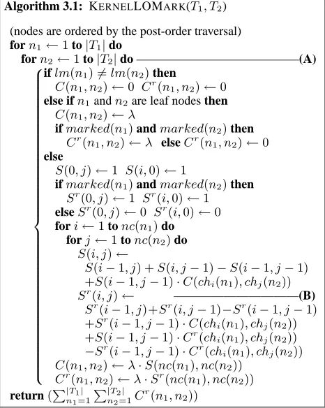
above kernels as well. Algorithm 3.1 shows the DP procedure for Klor, which is derived by extending the DP procedure forKlo (Kashima and Koyanagi, 2002). The key is the use of Cr(n1, n2), which
stores the sum over only marked subtrees, and its re-cursive calculation usingC(n1, n2)andCr(n1, n2)
[image:3.612.69.302.58.350.2](B). AnO(|T1||T2|) procedure for Kcr can also be derived by extending (Collins and Duffy, 2001).
Table 1: Malicious and non-malicious pairs in the 1k data (3,136 trees) used in Sec. 5.2. We used
K(Ti, Tj) = 104 with λ = 1as the threshold for
maliciousness. (A): pairs(i, i). (B): pairs from the same sentence except(i, i). (C): pairs from different sentences. Some malicious pairs are from different but similar sentences, which are difficult to detect.
Kr
lo Kcr
# pairs avg.K(Ti, Tj) # of pairs avg.K(Ti, Tj)
≥
104
(A) 3,121 1.17×1052
3,052 2.49×1032
(B) 7,548 7.24×1048 876 1.26×1032 (C) 6,510 6.80×10⁹
28 1.82×10⁴
<
104
(A) 15 4.19×10³ 84 3.06×10³ (B) 4,864 2.90×10²
11,536 1.27×10²
(C) 9,812,438 1.82×101
9,818,920 1.84×10⁻¹
4 Fast Training with Tree Kernels 4.1 Basic Idea
As mentioned, we define two types of tree pairs: ma-licious and non-mama-licious pairs. Table 1 shows how these two types of pairs are distributed in an actual training set. There is a clear distinction between ma-licious and non-mama-licious pairs, and we can exploit this property to speed up the training.
We define subset F = {Fi} (feature subtrees), which includes only the subtrees that appear as a common included subtree in the non-malicious pairs. We convert a tree to feature vectorV(Tj) = ³p
W(Fi)#Fi(Tj)
´
iusing onlyF. Then we use a procedure that chooses the DP procedure or the in-ner product procedure depending on maliciousness:
K(Ti, Tj) = (
K(Ti, Tj)(DP) if(i, j)is malicious.
hV(Ti), V(Tj)i otherwise
This procedure returns the same value as the origi-nal calculation. Naively, if|V(Ti)|(the number of feature subtrees such that #Fi(Ti) 6= 0) is small
enough, we can expect a speed-up because the cost of calculating the inner product is O(|V(Ti)| +
|V(Tj)|). However, since|V(Ti)|might increase as the training set becomes larger, we need a way to scale the speed-up to large data. In most kernel-based methods, such as SVMs, we actually need to calculate the kernel values with all the train-ing examples for a given example Ti: KS(Ti) =
{K(Ti, T1), . . . , K(Ti, TL)}, where L is the num-ber of training examples. Using occurrence
pre-Algorithm 4.1: CALCULATEKS(Ti)
for eachF such that #F(Ti)6= 0do
for each(j,#F(Tj))∈OP(F)do
KS(j)←KS(j) +W(F)·#F(Ti)·#F(Tj) (A)
forj= 1toLdo
if(i, j)is malicious thenKS(j)←K(Ti, Tj) (DP)
pared beforehand, we can calculate KS(Ti) effi-ciently (Algorithm 4.1). A similar technique was used in (Kudo and Matsumoto, 2003a) to speed up the calculation of inner products.
We can show that the per-pair cost of Algorithm 4.1 is O(c1Q+rmc2|Ti||Tj|), where Q is the av-erage number of common feature subtrees in a tree pair,rm is the rate of malicious pairs,c1 andc2 are
the constant factors for vector operations and DP op-erations. This cost is independent of the number of training examples. We expect from our observations that bothQandrmare very small and thatc1 ¿c2.
4.2 Feature Subtree Enumeration with Malicious Pair Detection
To detect malicious pairs and enumerate feature sub-treesF(and to convert each tree to a feature vector), we developed an algorithm based on the FREQT al-gorithm (Asai et al., 2002). The FREQT alal-gorithm can efficiently enumerate subtrees that are included (Definition 2.1) in more than a pre-specified number of trees in the training examples by generating can-didate subtrees using right most expansions (RMEs). FREQT-based algorithms have recently been used in methods that treat subtrees as features (Kudo and Matsumoto, 2004; Kudo and Matsumoto, 2003b).
To develop the algorithm, we made the defini-tion of maliciousness more search-oriented since it is costly to check for maliciousness based on the ex-act number of common subtrees or the kernel values (i.e., by using the DP procedure for all L2 pairs). Whatever definition we use, the correctness is pre-served as long as we do not fail to enumerate the subtrees that appear in the pairs we consider non-malicious. First, we consider pairs (i, i) to always be malicious. Then, we use a FREQT search that enumerates the subtrees that are included in at least two trees as a basis. Next, we modify FREQT so that it stops the search if candidate subtreeFiis too large (larger than sizeD, e.g., 20), and we regard the pairs of the trees whereFi appears as malicious because having a large subtree in common implies having a
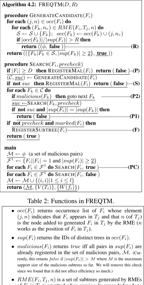
Algorithm 4.2: FREQTM(D, R)
procedure GENERATECANDIDATE(Fi)
for each(j, n)∈occ(Fi)do
for each(Fk, nr)∈RM E(Fi, Tj, n)do
S ← S ∪ {Fk}; occ(Fk)←occ(Fk)∪(j, nr)
if|occ(Fk)|/|sup(Fi)|> Rthen
return((φ, false))————————————(R) return(({Fk|Fk∈ S,|sup(Fk)| ≥2}, true))
procedure SEARCH(Fi, precheck)
if|Fi| ≥D then REGISTERMAL(Fi) return(false)–(P) (C, suc)←GENERATECANDIDATE(Fi)
if notsuc then REGISTERMAL(Fi) return(false)—(S)
for eachFk∈ Cdo
ifmalicious(Fk) then goto nextFk —————-(P2) suc←SEARCH(Fk, precheck)
if notsucand|sup(Fi)|=|sup(Fk)|then
return(false)——————————————–(P1) if notprecheckandmarked(Fi)then
REGISTERSUBTREE(Fi)————————————(F)
return(true)
main
M ←φ (a set of malicious pairs)
F1← {F
i||Fi|= 1and|sup(Fi)| ≥2}
for eachFi∈ F1do SEARCH(Fi, true)—————-(PC)
for eachFi∈ F1do SEARCH(Fi, false)
M ← M ∪ {(i, i)|1≤i≤l}
[image:4.612.310.547.55.523.2]return(M,{V(Ti)},{W(fi)})
Table 2: Functions in FREQTM.
• occ(Fi) returns occurrence list of Fi whose element (j, n)indicates thatFiappears inTjand thatn(ofTj)
is the node added to generatedFiinTjby the RME (n
works as the position ofFiinTj).
• sup(Fi)returns the IDs of distinct trees inocc(Fi).
• malicious(Fi)returnstrueiff all pairs insup(Fi)are
already registered in the set of malicious pairs,M. (Cur-rently, this returnsfalseif|sup(Fi)|> MwhereMis the maximum
support size of the malicious subtrees so far. We will remove this check since we found that it did not affect efficiency so much.)
• RM E(Fi, Tj, n)is a set of subtrees generated by RMEs
ofFiinTj(permitted when previously expanded node to
generateFiisn).
possibly exponential number of subtrees of that sub-tree in common. Although this test is heuristic and conservative in that it ignores the shape and marks of a tree, it works fine empirically.
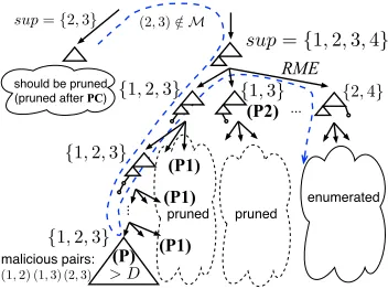
RME sincesup(Fk)⊆sup(Fi). This means we do not need to enumerateFinor any descendant ofFi.
• (P) Once|Fi| ≥ Dand the malicious pairs are registered, we stop searching further.
• (P1) If the search fromFk(expanded fromFi) found a malicious subtree and if|sup(Fi)| =
|sup(Fk)|, we stop the search from any other subtree Fm (expanded from Fi) since we can prove thatmalicious(Fm) =truewithout ac-tually testing it (proof omitted).
• (P2) If malicious(Fk) = true, we prune the search from Fk. To prune even when
malicious(Fk) becomes true as a result of
succeeding searches, we first run a search only for detecting malicious pairs (see (PC)).
• (S) We stop searching when the occurrence list becomes too long (larger than thresholdR) since it causes a severe search slowdown.
Note that we use a depth-first version of FREQT as a basis to first find the largest subtrees and to detect malicious pairs at early points in the search. Enu-meration of unnecessary subtrees is avoided because the registration of subtrees is performed at the post-order position (F). The conversion to vectors is per-formed by assigning an ID to subtreeFiwhen regis-tering it at (F) and distributing the ID to all the exam-ples inocc(Fi). Finally,Dshould be large enough to make rm sufficiently small but should not be so large that too many feature subtrees are enumerated. We expect that the cost of FREQTM is offset by the faster training, especially when training on the same data is repeatedly performed as in the tuning of hyperparameters.
ForKcr, we use a similar search procedure. How-ever, the RME is modified so that all the children of a CFG production are expanded at once. Although the modification is not trivial, we omit the explana-tion due to space limitaexplana-tions.
4.3 Feature Compression
Additionally, we use a simple but effective feature compression technique to boost speed-up. The idea is simple: feature subtreesFiandFj can be treated as one featurefk, with weightW(fk) = W(Fi) +
W(Fj) ifOP(Fi) = OP(Fj). This drastically re-duces the number of features. Although this is
sim-sup={1,2,3,4} sup={2,3} (2,3)∈ M/
(1,2)(1,3) (2,3)
{1,2,3}
{1,2,3}
{1,2,3}
{1
,3} {2,4}
> D
[image:5.612.339.515.57.188.2]
Figure 3: Pruning in FREQTM.
ilar to finding closed and maximal subtrees (Chi et al., 2004), it is easy to implement since we need only the occurrence pattern,OP(Fi), which is easily ob-tained fromocc(Fi)in the FREQTM search.
4.4 Alternative Methods
Vishwanathan and Smola (2004) presented the
O(|T1|+|T2|) procedure that exploits suffix trees
to speed up the calculation of tree kernels. However, it can be applied to only a few types of subtrees that can be represented as a contiguous part in a string representation of a tree. Therefore, neitherKlor nor
Kcrcan be sped up by using this procedure.
Another method is to change an inner loop, such as (B) in Algorithm 3.1, so that it iterates only over nodes inT2that havel(n1). We use this as the
base-line for comparison, since we found that this is about two times faster than the standard implementation.1
4.5 Remaining Problem
Note that the method described here cannot speed up classification, since the converted vectors are valid only for calculating the kernels between trees in the training set. However, when we classify the same trees repeatedly, we can convert the trees in the train-ing set and the classified trees at the same time and use the obtained vectors for classification.
5 Evaluation
We first evaluated the speed-up by our method for the semantic role labeling (SRL) task. We then demonstrated that the speed-up method enables a de-tailed comparison ofKlor andKcrfor the SRL task.
1ForKr
c, it might be possible to speed up comparisons in
Table 3: Conversion statistics and speed-up for semantic role A2. Kr
lo Kcr
size (# positive examples) 1,000 2,000 4,000 8,000 12,000 1,000 2,000 4,000 8,000 12,000 # examples 3,136 6,246 12,521 25,034 34,632 3,136 6,246 12,521 25,034 34,632 # feature subtrees (×104
) 804.4 2,427.3 6,542.9 16,750.1 26,146. 5 3.473 9.009 21.867 52.179 78.440 # features (compressed) (×104
) 20.7 67.3 207.2 585.9 977.0 0.580 1.437 3.426 8.128 12.001 avg.|V|(compressed) 468.0 866.5 1,517.3 2,460.5 3,278.3 10.5 14.0 17.9 23.1 25.9 rate of malicious pairsrm(%) 0.845 0.711 0.598 0.575 1.24 0.161 0.0891 0.0541 0.0370 0.0361
conversion time (sec.) 208.0 629.2 1,921.1 6,519.8 14,824.9 3.8 8.7 20.4 46.5 70.4 SVM time (DP+lookup) (sec.) 487.9 1,716.2 4,526.4 79,800.7 92,542.2 360.7 1,263.5 5,893.3 53,055.5 47,089.2 SVM time (proposed) (sec.) 17.5 68.6 186.4 1,721.7 2,531.8 4.9 25.7 119.5 982.8 699.1 speed-up factor 27.8 25.0 24.3 46.4 36.6 73.3 49.1 49.3 53.98 67.35
5.1 Setting
We used the data set provided for the CoNLL05 SRL shared task (Carreras and M`arquez, 2005). We used only the training part and divided it into our training, development, and testing sets (23,899, 7,966, and 7,967 sentences, respectively). As the tree structure, we used the output of Collins’ parser (with WSJ-style non-terminals) provided with the data set. We also used POS tags by inserting the nodes labeled by POS tags above the word nodes. The average num-ber of nodes in a tree was about 82. We ignored any arguments (and verbs) that did not match any node in the tree (the rate of such cases was about 3.5%).2 The words were lowercased.
We used TinySVM3 as the implementation of SVM and added our tree kernels,Klor andKcr. We implemented FREQTM based on the implementa-tion of FREQT by Kudo.4 We normalized the kernel values: K(Ti, Tj)/
p
K(Ti, Ti)×K(Tj, Tj). Note that this normalization barely affected the training time since we can calculateK(Ti, Ti)beforehand.
We assumed two-step labeling where we first find the argument node and then we determine the label by using a binary classifier for each semantic role. In this experiment, we focused on the performance for the classifiers in the latter step. We used the marked labeled ordered tree that encoded the target role as a positive example and the trees that encoded other roles of the verb in the same sentence as negative examples. We trained and evaluated the classifiers using the examples generated as above.5
2
This was caused by parse errors, which can be solved by us-ing more accurate parsers, and by bracketus-ing inconsistencies be-tween parser outputs and SRL annotations (e.g., phrasal verbs), many of which can be avoided by using heuristic transformers.
3
http://chasen.org/˜taku/software/TinySVM
4
http://chasen.org/˜taku/software/freqt
5The evaluation is slightly easier since the classifier for role
5.2 Training Speed-up
We calculated the statistics for the conversion by FREQTM and measured the speed-up in SVM train-ing for semantic role A2, for various numbers of training examples. For FREQTM, we usedD= 20
andR = 20. For SVM training, we used conver-gence tolerance0.001(-e option in TinySVM), soft margin cost C = 1.0×10³ (-c), maximum
num-ber of iterations 105, kernel cache size 512 MB (-m), and decay factor λ = 0.2 for the weight of each subtree. We compared the time with our fast method (Algorithm 4.1) with that with the DP pro-cedure with the node lookup described in Section 4.4. Note that these two methods yield almost iden-tical SVM models (there are very slight differences due to the numerical computation). The time was measured using a computer with 2.4-GHz Opterons. Table 3 shows the results for Klor andKcr. The proposed method made the SVM training substan-tially faster for bothKlor andKcr. As we expected, the speed-up factor did not decrease even though|V| increased as the amount of data increased. Note that FREQTM actually detected non-trivial mali-cious pairs such as those from very similar sentences in addition to trivial ones, e.g.,(i, i). FREQTM con-version was much faster and the converted feature vectors were much shorter forKcr, presumably be-causeKcrrestricts the subtrees more.
The compression technique described in Section 4.3 greatly reduced the number of features. Without this compression, the storage requirement would be impractical. It also boosted the speed-up. For ex-ample, the training time withKr
lofor the size 1,000 data in Table 3 was 86.32 seconds without compres-sion. This means that the compression boosted the
100 101 102 103 104 105
103 104
Time (sec.)
Number of examples conversion SVM (DP+lookup) SVM (proposed)
100 101 102 103 104 105
103 104
Time (sec.)
[image:7.612.81.292.57.137.2]Number of examples conversion SVM (DP+lookup) SVM (proposed)
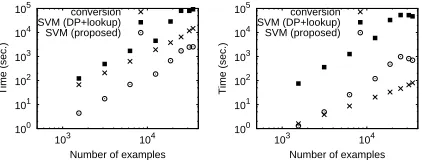
Figure 4: Scaling of conversion time and SVM train-ing time. Left:Klor. Right:Kcr
0 2 4 6 8 10 12 14
5 10 15 20 25 30 0 0.2 0.4 0.6 0.8 1
Time (
×
10
3 sec.)
Malicious Pair Rate (r
m
)
D conversion SVM (proposed) rm
0 0.2 0.4 0.6 0.8 1
5 10 15 20 25 30 0 0.2 0.4 0.6 0.8 1
Time (
×
10
3 sec.)
Malicious Pair Rate (r
m
)
[image:7.612.73.297.179.252.2]D conversion SVM (proposed) rm
Figure 5: Relation betweenDand conversion time, SVM training time, andrm. Left:Klor. Right:Kcr
speed-up by a factor of more than 5.
The cost of FREQTM is much smaller than that of SVM training with DP. Therefore, our method is beneficial even if we train the SVM only once.
To see how our method scales to large amounts of data, we plotted the time for the conversion and the SVM training w.r.t. data size on a log-log scale. As shown in Figure 4, the scaling factor was about 1.7 for the conversion time, 2.1 for SVM training with DP, and 2.0 for the proposed SVM training for
Kr
lo. ForKcr, the factors were about 1.3, 2.1, and 2.0, respectively. Regardless of the method, the cost of SVM training was about O(L2), as reported in the literature. Although FREQTM also has a super-linear cost, it is smaller than that of SVM training. Therefore, the cost of SVM training will become a problem before the cost of FREQTM does.
As we mentioned, the choice of Dis a trade-off. Figure 5 shows the relationships betweenDand the time of conversion by FREQTM, the time of SVM training using the converted vectors, and the rate of malicious pairs,rm. We can see that the choice ofD is more important in the case ofKloand thatD= 20 used in our evaluation is not a bad choice.
5.3 Semantic Role Labeling
We assessed the performance ofKlor andKcrfor se-mantic roles A1, A2, AM-ADV, and AM-LOC us-ing our fast trainus-ing method. We tuned soft mar-gin costC andλby using the development set (we
used the technique described in Section 4.5 to en-able fast classification of the development set). We experimented with two training set sizes (4,000 and 8,000). For eachλ(0.1, 0.15, 0.2, 0.25, and 0.30), we tested 40 different values ofC (C ∈ [2. . .103] for size 4,000 andC ∈[0.5. . .103]for size 8,000), and we evaluated the accuracy of the best setting for the test set.6 Fast training is crucial since the per-formance differs substantially depending on the val-ues of these hyperparameters. Table 4 shows the re-sults. The accuracies are shown byF1. We can see
thatKlor outperformedKcr in all cases, presumably becauseKcr allows only too restrictive subtrees and therefore causes data sparseness. In addition, as one would expect, larger training sets are beneficial.
6 Discussion
The proposed speed-up method can also be applied to labeled ordered trees (e.g., for parse selection). However, the speed-up might be smaller since with-out node marks the number of subtrees increases while the DP procedure becomes simpler. On the other hand, the FREQTM conversion for marked la-beled ordered trees might be made faster by exploit-ing the mark information for prunexploit-ing. Although our method is not a complete solution in a classification setting, it might be in a clustering setting (in a sense it is training only). However, it is an open question whether unbalanced similarity, which is the key to our speed-up, is ubiquitous in NLP tasks and under what conditions our method scales better than the SVMs or other kernel-based methods.
Several studies claim that learning using tree ker-nels and other convolution kerker-nels tends to overfit and propose selecting or restricting features (Cumby and Roth, 2003; Suzuki et al., 2004; Kudo and Mat-sumoto, 2004). Sometimes, the classification be-comes faster as a result (Suzuki et al., 2004; Kudo and Matsumoto, 2004). We do not disagree with these studies. The fact that smallλvalues resulted in the highest accuracy in our experiment implies that too large subtrees are not so useful. However, since this tendency depends on the task, we need to assess the performance of full tree kernels for comparison. In this sense, our method is of great importance.
Node relation labeling is a generalization of node
6We used106
Table 4: Comparison betweenKr
loandKcr.
training set size = 4,000 training set size = 8,000
best setting F1(dev) F1(test) best setting F1(dev) F1(test)
A1 K
r
lo λ= 0.2,C= 13.95 87.89 87.90 λ= 0.25,C= 8.647 89.80 89.81 Kr
c λ= 0.15,C= 3.947 85.36 85.56 λ= 0.2,C= 17.63 87.93 87.96
A2 K
r
lo λ= 0.20,C= 13.95 85.65 84.70 λ= 0.20,C= 57.82 87.94 87.26 Kr
c λ= 0.10,C= 7.788 84.79 83.51 λ= 0.15,C= 1.0×10³ 87.37 86.23
AM-ADV K
r
lo λ= 0.25,C= 8.647 86.20 86.64 λ= 0.15,C= 45.60 86.91 87.01 Kr
c λ= 0.20,C= 3.344 83.58 83.72 λ= 0.20,C= 2.371 84.34 84.08
AM-LOC K
r
lo λ= 0.15,C= 20.57 91.11 92.92 N/A Kr
c λ= 0.15,C= 13.95 89.59 91.32 AM-LOC does not have more than 4,000 positive examples.
marking where we determine the mark (tag) of a node. Kashima and Koyanagi (2002) dealt with this task by inserting the node representing the mark above the node to be tagged and classifying the transformed tree using SVMs with tree kernels such asKlo. For the SRL task, Moschitti (2004) applied the tree kernel (Kc) to tree fragments that are heuris-tically extracted to reflect the role of interest. For re-lation extraction, Culotta and Sorensen (2004) pro-posed a tree kernel that operates on only the smallest tree fragment including two entities for which a re-lation is assigned. Our kernels on marked labeled ordered trees differ in what subtrees are permitted. Although comparisons are needed, we think our ker-nels are intuitive and general.
There are many possible structures for which tree kernels can be defined. Shen et al. (2003) proposed a tree kernel for LTAG derivation trees to focus only on linguistically meaningful structures. Culotta and Sorensen (2004) proposed a tree kernel for depen-dency trees. An important future task is to find suit-able structures for each task (the SRL task in our case). Our speed-up method will be beneficial as long as there is unbalanced similarity.
7 Conclusion
We have presented a method for speeding up the training with tree kernels. Using the SRL task, we demonstrated that our speed-up method made the training substantially faster.
References
T. Asai, K. Abe, S. Kawasoe, H. Arimura, H. Sakamoto, and S. Arikawa. 2002. Efficient substructure discov-ery from large semi-structured data. In SIAM SDM’02.
X. Carreras and L. M`arquez. 2005. Introduction to the CoNLL-2005 shared task: Semantic role labeling. In
CoNLL 2005.
Y. Chi, Y. Yang, Y. Xia, and R. R. Muntz. 2004. CMTreeMiner: Mining both closed and maximal fre-quent subtrees. In PAKDD 2004.
M. Collins and N. Duffy. 2001. Convolution kernels for natural language. In NIPS 2001.
A. Culotta and J. Sorensen. 2004. Dependency tree ker-nels for relation extraction. In ACL 2004.
C. Cumby and D. Roth. 2003. On kernel methods for relational learning. In ICML 2003.
D. Gildea and D. Jurafsky. 2002. Automatic labeling of semantic roles. Computational Linguistics, 28(3).
K. Hacioglu, S. Pradhan, W. Ward, J. H. Martin, and D. Jurafsky. 2004. Semantic role labeling by tagging syntactic chunks. In CoNLL 2004.
H. Kashima and T. Koyanagi. 2002. Kernels for semi-structured data. In ICML 2002, pages 291–298.
T. Kudo and Y. Matsumoto. 2003a. Fast methods for kernel-based text analysis. In ACL 2003.
T. Kudo and Y. Matsumoto. 2003b. Subtree-based Markov random fields and its application to natural language analysis (in Japanese). IPSJ, NL-157.
T. Kudo and Y. Matsumoto. 2004. A boosting algorithm for classification of semi-structured text. In EMNLP
2004, pages 301–308.
A. Moschitti. 2004. A study on convolution kernels for shallow semantic parsing. In ACL 2004.
L. Shen, A. Sarkar, and A. K. Joshi. 2003. Using LTAG based features in parse reranking. In EMNLP 2003.
J. Suzuki, H. Isozaki, and E. Maeda. 2004. Convolu-tion kernels with feature selecConvolu-tion for natural language processing tasks. In ACL 2004, pages 119–126.
V. Vapnik. 1995. The Nature of Statistical Learning
The-ory. Springer Verlag.
S. V. N. Vishwanathan and A. J. Smola. 2004. Fast ker-nels for string and tree matching. Kerker-nels and