Confidence in Structured Prediction Using Confidence Weighted Models

(1)

Confidence in Structured-Prediction using Confidence-Weighted Models

Avihai Mejer

Department of Computer Science Technion-Israel Institute of Technology

Haifa 32000, Israel

[email protected]

Koby Crammer

Department of Electrical Engineering Technion-Israel Institute of Technology

Haifa 32000, Israel

[email protected]

Abstract

Confidence-Weighted linear classifiers (CW) and its successors were shown to perform well on binary and multiclass NLP prob-lems. In this paper we extend the CW ap-proach for sequence learning and show that it achieves state-of-the-art performance on four noun phrase chucking and named entity

recog-nition tasks. We then derive few

algorith-mic approaches to estimate the prediction’s correctness of each label in the output se-quence. We show that our approach provides a reliable relative correctness information as it outperforms other alternatives in ranking label-predictions according to their error. We also show empirically that our methods output close to absolute estimation of error. Finally, we show how to use this information to im-prove active learning.

1 Introduction

In the past decade structured classification has seen much interest by the machine learning community. After the introduction of conditional random fields (CRFs) (Lafferty et al., 2001), and maximum mar-gin Markov networks (Taskar et al., 2003), which are batch algorithms, new online method were in-troduced. For example the passive-aggressive algo-rithm was adapted to chunking (Shimizu and Haas, 2006), parsing (McDonald et al., 2005b), learning preferences (Wick et al., 2009) and text segmenta-tion (McDonald et al., 2005a). These new online algorithms are fast to train and simple to implement, yet they generate models that output merely a

pre-diction with no additional information, as opposed to probabilistic models like CRFs or HMMs.

In this work we fill this gap proposing few al-ternatives to compute confidence in the output of discriminative non-probabilistic algorithms. As be-fore, our algorithms output the highest-scoring beling. However, they also compute additional la-belings, that are used to compute theper word con-fidence in its labelings. We build on the recently introduced confidence-weighted learning (Dredze et al., 2008; Crammer et al., 2009b) and induce a dis-tribution over labelings from the disdis-tribution main-tained over weight-vectors.

We show how to compute confidence estimates in the label predicted per word, such that the con-fidence reflects the probability that the label is not correct. We then use this confidence information to rank all labeled words (in all sentences). This can be thought of as a retrieval of the erroneous words, which can than be passed to human anno-tator for an examination, either to correct these mis-takes or as a quality control component. Next, we show how to apply our techniques to active learning over sequences. We evaluate our methods on four NP chunking and NER datasets and demonstrate the usefulness of our methods. Finally, we report the performance of obtained by CW-like adapted to se-quence prediction, which are comparable with cur-rent state-of-the-art algorithms.

2 Confidence-Weighted Learning

Consider the following online binary classification problem that proceeds in rounds. On the ith round the online algorithm receives an inputxi ∈ Rdand

(2)

applies its current rule to make a predictionyˆi ∈ Y, for the binary set Y = {−1,+1}. It then receives the correct labelyi ∈ Y and suffers a loss`(yi,yˆi). At this point, the algorithm updates its prediction rule with the pair (xi, yi) and proceeds to the next round. A summary of online algorithms can be found in (Cesa-Bianchi and Lugosi, 2006).

Online confidence-weighted (CW) learning (Dredze et al., 2008; Crammer et al., 2008), generalized the passive-aggressive (PA) update principle to multivariate Gaussian distributions over the weight vectors - N (µ,Σ) - for binary classification. The mean µ ∈ _Rd _{contains the} current estimate for the best weight vector, whereas the Gaussian covariance matrixΣ∈ _Rd×d_captures the confidence in this estimate. More precisely, the diagonal elements Σp,p, capture the confidence in the value of the corresponding weight µ_p ; the smaller the value of Σp,p, is, the more confident is the model in the value of µ_p. The off-diagonal elements Σp,q for p 6= q capture the correlation between the values of µ_p andµ_q. When the data is of large dimension, such as in natural language processing, a model that maintains a full covariance matrix is not feasible and we back-off to diagonal covariance matrices.

CW classifiers are trained according to a PA rule that is modified to track differences in Gaussian dis-tributions. At each round, the new mean and co-variance of the weight vector distribution is chosen to be the solucion of an optimization problem (see (Crammer et al., 2008) for details). This particu-lar CW rule may over-fit by construction. A more recent alternative scheme called AROW (adaptive regularization of weight-vectors) (Crammer et al., 2009b) replaces the guaranteed prediction at each round with the a more relaxed objective (see (Cram-mer et al., 2009b)). AROW has been shown to perform well in practice, especially for noisy data where CW severely overfits.

The solution for the updates of CW and AROW share the same general form,

µ_i₊₁=µ_i+αiΣiyixi; Σ−i+11 = Σ −1

i+1+βixix>i , (1)

where the difference between CW and AROW is the specific instance-dependent rule used to set the val-ues ofαiandβi.

Algorithm 1Sequence Labeling CW/AROW Input:Joint feature mappingΦ(x,y)∈_Rd

Initial variancea >0

Tradeoff Parameterr >0(AROW) or Confidence parameterφ(CW) Initialize: µ₀ =0,Σ0=aI

fori= 1,2. . . do Getxi ∈ X

Predict best labeling ˆ

y_i= arg maxzµi−1·Φ(xi,z)

Get correct labelingy_i∈ Y|xi| Define∆i,y,yˆ =Φ(x,yi)−Φ(x,yˆi)

Compute αi and βi (Eq. (3) for CW ; Eqs. (4),βi= 1/r) for AROW)

Setµ_i =µ_i−1+αiΣi−1∆i,y,ˆy

SetΣ−_i 1 = Σ−_i₋1₁+βi∆i,y,ˆy∆>i,y,yˆ

end for

3 Sequence Labeling

In the sequence labeling setting, instances x be-long to a general input spaceX and conceptually are composed of a finite numbernof components, such as words of a sentence. The number of components n = |x|varies between instances. Each part of an instance is labelled from a finite setY, |Y| = K. That is, a labeling of an entire instance belongs to the product sety∈ Y × Y. . .Y(ntimes).

We employ a general approach (Collins, 2002; Crammer et al., 2009a) to generalize binary clas-sification and use a joined feature mapping of an instancex and a labelingy into a common vector space,Φ(x,y)∈_Rd_.

Given an input instance xand a modelµ ∈ _Rd we predict the labeling with the highest score,yˆ = arg maxzµ·Φ(x,z). A brute-force approach

eval-uates the value of the scoreµ·Φ(x,z)for each pos-sible labelingz ∈ Yn_{, which is not feasible for large} values ofn. Instead, we follow standard factoriza-tion and restrict the joint mapping to be of the form,

Φ(x,y) =Pn_p₌₁Φ(x, yp) +Pnq=2Φ(x, yq, yq−1).

That is, the mapping is a sum of mappings, each tak-ing into consideration only a label of a stak-ingle part, or two consecutive parts. The time required to compute themax operator is linear innand quadratic inK using the dynamic-programming Viterbi algorithm.

(3)

the current labeled instance (xi,y_i) to update the model. We now define the update rule both for a version of CW and for AROW for strucutred learn-ing, staring with CW. Given the input parameterφ of CW we denote by φ0 = 1 +φ2/2, φ00= 1 +φ2. We follow a similar argument as in the single up-date of (Crammer et al., 2009a, sec. 5.1) to se-quence labeling by a reduction to binary classifica-tion. We first define the difference between the fea-ture vector associated with the current labeling y_i and the feature vector associated with some label-ing z to be, ∆i,y,z = Φ(x,yi)−Φ(x,z) , and in particular, when we use the predictionyˆ_i we get,

∆i,y,yˆ =Φ(x,yi)−Φ(x,yˆi).The CW update is,

µ_i=µ_i₋₁+αiΣi−1∆i,y,yˆ

Σ−_i 1= Σ−_i₋1₁+βi∆i,y,yˆ∆>i,y,yˆ , (2)

where the two scalars αi and βi are set using the update rule defined by (Crammer et al., 2008) for binary classification,

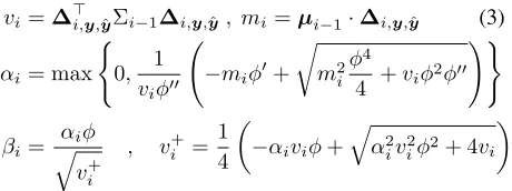
vi=∆>i,y,ˆyΣi−1∆i,y,yˆ, mi =µi−1·∆i,y,yˆ (3)

αi= max

(

0, 1

viφ00

−miφ0+

r

m2 i

φ4

4 +viφ

2_φ00

!)

βi=

αiφ

q v_i+

, v_i+= 1 4

−αiviφ+

q α2

ivi2φ2+ 4vi

2

We turn our attention and describe a mod-ification of AROW for sequence prediction. Replacing the binary-hinge loss in (Crammer et al., 2009b, Eqs. (1,2)) the first one with the corresponding multi-class hinge loss for structured problems we obtain, 1₂(µ_i−µ)>Σ−_i 1(µ_i−µ) +

1

2r(max{0,maxz6=y{d(y,z)−µ·(∆i,y,z)}})

2 ,

where, d(y,z) = P|x|

q=11yq6=zq , is the hamming distance between the two label sequencesyandz. The last equation is hard to optimize since the max operator is enumerating over exponential number of possible labellingsz. We thus approximate the enu-meration over all possiblezwith the predicted label sequence yˆi and get, 1₂(µi−µ)

>

Σ−_i1(µ_i−µ) +

1 2r max

0, d(y_i,yˆ_i)−µ· ∆i,y,ˆy 2

. Com-puting the optimal value of the last equation we get an update of the form of the first equation of Eq. (2) where

αi = max

0, d(y_i,yˆ_i)−µ_i₋₁· ∆i,y,yˆ r+∆>_i,_y_,_ˆ_yΣi−1∆i,y,yˆ

. (4)

[image:3.612.316.542.53.203.2]

Dataset Sentences Words Features NP chunking 11K 259K 1.35M NER English 17.5K 250K 1.76M NER Spanish 10.2K 317.6K 1.85M NER Dutch 21K 271.5K 1.76M

Table 1: Properties of datasets.

AROW CW 5-best PA Perceptron NP chunking 0.946 0.947 0.946 **0.944 NER English 0.878 0.877 * 0.870 * 0.862 NER Dutch 0.791 0.787 0.784 * 0.761 NER Spanish 0.775 0.774 0.773 * 0.756

Table 2: Averaged F-measure of methods. Statistical sig-nificance (t-test) are with respect to AROW, where * in-dicates 0.001 and ** inin-dicates 0.01

We proceed with the confidence paramters in (Crammer et al., 2009b, Eqs. (1,2)), which takes into considiration the change of confidence due to the up-date. The effective features vector that is used to update the mean parameters is∆i,y,yˆ, and thus the

structured update is,1₂logdet Σi

det Σ

+1₂Tr Σ−_i₋1₁Σ +

1 2r∆

>

i,y,yˆΣ∆i,y,yˆ . Solving the above equation we

get an update of the form of the second term of Eq. (2) whereβi = 1_r . The pseudo-code of CW and AROW for sequence problems appears in Alg. 1.

4 Evaluation

For the experiments described in this paper we used four large sequential classification datasets taken from the CoNLL-2000, 2002 and 2003 shared tasks: noun-phrase (NP) chunking (Kim et al., 2000), and named-entity recognition (NER) in Spanish, Dutch (Tjong and Sang, 2002) and English (Tjong et al., 2003). The properties of the four datasets are summarized in Table 1. We followed the feature generation process of (Sha and Pereira, 2003).

[image:3.612.72.302.328.414.2]

(4)

0.934 0.936 0.938 0.94 0.942 0.944 0.936

0.938 0.94 0.942 0.944 0.946 0.948

Recall

Precision

Perceptron PA CW AROW

(a) NP Chunking

0.81 0.82 0.83 0.84 0.85 0.86 0.82

0.83 0.84 0.85 0.86 0.87 0.88 0.89

Recall

Precision

(b) NER English

0.68 0.7 0.72 0.74 0.76 0.7

0.72 0.74 0.76 0.78 0.8

Recall

Precision

(c) NER Dutch

0.7 0.72 0.74 0.76 0.7

0.72 0.74 0.76 0.78

Recall

Precision

[image:4.612.93.534.61.165.2]

(d) NER Spanish

Figure 1:Precision and Recall on four datasets (four panels). Each connected set of ten points corresponds to the performance of

a specific algorithm after each of the 10 iterations, increasing from bottom-left to top-right.

Prec Recall F-meas % Err CW 0.945 0.942 0.943 2.34% NP chunking

CRF 0.938 0.934 0.936 2.66%

CW 0.838 0.826 0.832 3.38% NER English

CRF 0.823 0.820 0.822 3.53%

CW 0.803 0.755 0.778 2.05% NER Dutch

CRF 0.775 0.753 0.764 2.09%

CW 0.738 0.720 0.729 4.09% NER Spanish

CRF 0.751 0.730 0.740 2.05%

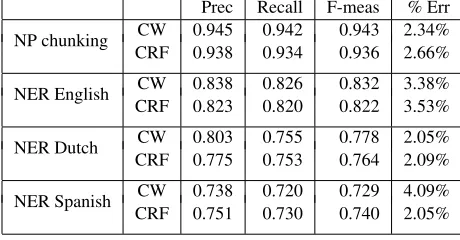
Table 3: Precision, Recall, F-measure and percentage of mislabeled words results of CW vs. CRF

setting. Three options are possible: compute a fullΣ and then take its diagonal elements; compute a full inverseΣ, take its diagonal elements and then com-pute its inverse; assume thatΣis diagonal and com-pute the optimal update for this choice. We found the first method to work best, and thus employ it from now on.

The hyper parameters (rfor AROW,φfor CW,C for PA) were tuned for each task by a single run over a random split of the data into a three-fourths train-ing set and a one-fourth test set. We used parameter averaging with all methods.

For each of the four datasets we used 10-fold cross validation. All algorithms (Perceptron, PA, CW and AROW) are online, and as mentioned above work in rounds. For each of the ten folds, each of the four algorithm performed ten (10) iterations over the training set and the performance (Recall, Precision and F-measure) was evaluated on the test set after each iteration.

The F-measure of the four algorithms after 10 it-erations over the four datasets is summarized in Ta-ble 2. The general trend is that AROW slightly out-performs CW, which is better than PA that is

bet-ter than the Perceptron. The difference between AROW and the Perceptron is significant, and be-tween AROW and PA is significant in two datasets. The difference between AROW and CW is not sig-nificant although it is consistent.

We further investigate the convergence properties of the algorithms in Fig. 1. The figure shows the re-call and precision results after each training round averaged across the 10 folds. Each panel summa-rizes the results on a single dataset, and in each panel a single set of connected points corresponds to one algorithm. Points in the left-bottom of the plot cor-respond to early iterations and points in the right-top correspond to later iterations. Long segments indi-cate a big improvement in performance between two consecutive iterations.

Few points are in order. First, high (in the y-axis) values indicate better precision and right (in the x-axis) values indicate better recall. Second, the per-formance of all algorithms is converging in about10 iterations as indicated by the fact the points in the top-right of the plot are close to each other. Third, the long segments in the bottom-left for the Percep-tron algorithm indicate that this algorithm benefits more from more than one pass compared with the other. Fourth, on the three NER datasets after 10 it-erations AROW gets slightly higher precision values than CW, while CW gets slightly higher recall val-ues than AROW. This is indicated by the fact that the right red square is left and above to the top-right blue circle. Finally, in two datasets, PA get slightly better recall than CW and AROW, but pay-ing in terms of precision and overall F-measure per-formance.

[image:4.612.71.301.207.327.2]

(5)

algo-NP chunking NER English NER Spanish NER Dutch 0

0.05 0.1 0.15 0.2 0.25 0.3 0.35 0.4 0.45 0.5 0.55

CRF KD−Fixed (K=50) KD−PC (K=50) Delta WKBV (K=30) KBV (K=30) Random

(a) AvgP CW & CRF

NP chunkingNER English NER Spanish NER Dutch 0

0.02 0.04 0.06 0.08 0.1

Root Mean Squared Error in Confidence

CRF KD−Fixed (K=50) KD−PC (K=50) WKBV (K=30)

(b) RMSE CW & CRF

NP chunkingNER English NER Spanish NER Dutch 0

0.05 0.1 0.15 0.2 0.25 0.3 0.35 0.4 0.45 0.5 0.55

KD−Fixed (K=50) Delta WKBV (K=30) KBV (K=30) Random

(c) AvgP PA

NP chunking0 NER English NER Spanish NER Dutch 0.02

0.04 0.06 0.08 0.1

Root Mean Squared Error in Confidence

KD−Fixed (K=50) WKBV (K=30)

[image:5.612.75.295.53.268.2]

(d) RMSE PA

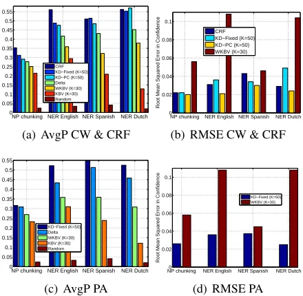
Figure 2: Two left panels: average precision of rankings of

the words of the test-set according to confidence in the predic-tion of seven methods (left to right bars in each group): CRF, KD-Fixed, KD-PC, Delta, WKBV, KBV and random ordering, when training with the CW algorithm (top) and the PA algo-rithm (bottom). Two right panels: The root-mean-squared-error of four methods that output absolute valued confidence: CRF, KD-Fixed, KD-PC and WKBV.

rithm which is a batch algorithm. We used Mal-let toolkit (McCallum, 2002) for CRF implementa-tion. For feature generation we used a combination of standard methods provided with Mallet toolkit (called pipes). We chose a combination yielding a feature set that is close as possible to the feature set we used in our system but it was not a perfect match, CRF generated about20%fewer features in all datasets. Nevertheless, any other combination of pipes we tried only hurt CRF performance. The pre-cision, recall, F-measure and percentage of misla-beled words of CW algorithm compared with CRF measured over a single split of the data into a three-fourths training set and a one-fourth test set is sum-marized in Table 3. We see that in three of the four datasets CW outperforms CRF and in one dataset CRF performs better. Some of the performance dif-ferences may be due to the difdif-ferences in features.

5 Confidence in the Prediction

Most large-margin-based training algorithms output models that their prediction is a single labeling of the input, with no additional confidence information about the correctness of that prediction. This

situ-ation is acceptable when the output of the system is used anyway, irrespectively of its quality. This situation is not acceptable when the output of the system is used as an input of another system that is sensitive to correctness of the specific prediction or that integrates various input sources. In such cases, additional confidence information about the correct-ness of these feeds for specific input can be used to improve the total output quality. Another case where such information is useful, is when there is additional agent that is validating the output of the system. The confidence information can be used to direct the check into small number of suspected predictions as opposed to random check, which may miss errors if their rate is small.

Some methods only provide relative confidence information. This information can be used torank

all predictions according to their confidence score, which can be used to direct a quality control com-ponent to detect errors in the prediction. Note, the confidence score is meaningless by itself and in fact, any monotonic transformation of the con-fidence scores yield equivalent concon-fidence informa-tion. Other methods are providing confidence in the predicted output as anabsoluteinformation, that is, the probability of a prediction to be correct. We re-fer to these probabilistic outputs in a frequentists ap-proach. When taking a large set of events (predic-tions) with similar probability confidence valueνof being correct, we expect that aboutνfraction of the predictions in the group will be correct.

Algorithms: All of our methods to evaluate confi-dence, except two (Delta and CRF below), share the same conceptual approach and work in two stages. First, a method generates a set ofKpossible label-ings for the input sentence (instead of a single pre-diction). Then, the confidence in a predicted label-ing for a specific word is defined to be the proportion of labelings which are consistent with the predicted label. Formally, letz(i) _for_i _{= 1}_{. . . K} _{be the} _K

labelings for some inputx, and let yˆ be the actual prediction for the input. (We do not assume that ˆ

y = z(i) _{for some}_i_{). The confidence in the label}

ˆ

ypof wordp= 1. . .|x|is defined to be

(6)

1000 2000 3000 4000 5000 0 200 400 600 800 1000 Word Index

No. of Words Classified Incorrectly

CRF KBV (K=30) WKBV (K=30) KD−PC (K=50) KD−Fixed (K=50) Delta Random

(a) NP Chunking

1000 2000 3000 4000 5000 0 200 400 600 800 1000 1200 1400 1600 Word Index

(b) NER English

1000 2000 3000 4000 5000 0 200 400 600 800 1000 1200 1400 Word Index

(c) NER Dutch

1000 2000 3000 4000 5000 0

500 1000 1500

Word Index

(d) NER Spanish

1000 2000 3000 4000 5000 −100 −50 0 50 100 150 200 250 Word Index

(e) NP Chunking

1000 2000 3000 4000 5000 −100 −50 0 50 100 150 200 250 300 Word Index

(f) NER English

1000 2000 3000 4000 5000 −100 −50 0 50 100 Word Index

(g) NER Dutch

1000 2000 3000 4000 5000 −100 −50 0 50 100 150 200 Word Index

[image:6.612.87.527.59.264.2]

(h) NER Spanish

Figure 3:Total number of detected erroneous words vs. the number of ranked words (top panels), and relative to the Delta method

(bottom panels). In other words, the lines in the bottom panels are the number ofadditionalerroneous words detected compared to Delta method. All methods builds on the same weight-vector except CRF (see text).

We tried four approaches to generate the set of K possible labelings. The first method is valid only for methods that induce a probability distribution over predicted labels. In this case, we drawK la-belings from this distribution. Specifically, we ex-ploit the Gaussian distribution over weight vectors w ∼ N(µ,Σ)maintained by AROW and CW, by inducing a distribution over labelings given an in-put. The algorithm samples K weight vectors ac-cording to this Gaussian distribution and outputs the best labeling with respect to each weight vector. For-mally, we define the set Z = {z(i) : z(i) = arg maxzw·Φ(x,z)wherew∼ N(µ,Σ)}

The predictions of algorithms that use the mean weight vectoryˆ = arg maxzµ·Φ(x,z)are

invari-ant to the value of the inputΣ(as noted by (Cram-mer et al., 2008)). However for the purpose of con-fidence estimation the specific value ofΣhas a huge affect. Small eigenvalue ofΣyield that all the ele-ments ofZwill be the same, while large values yield random elements in the set, ignoring the input.

One possible simple option is to run the algorithm few times, with few possible initializations ofΣand choose one using the training set. However since the actual predictions of all these versions is the same (invariance to scaling, see (Crammer et al., 2008)) in practice we run the algorithm once initializing Σ = I. Then, after the training is completed, we

try few scalings of the final covariancesΣfor some positive scalars, and choose the best valuesusing the training set. We refer to this method asKD-PC

for K-Draws by Parameters Confidence.

The second method to estimate confidence fol-lows the same conceptual steps, except that we used an isotropic covariance matrix, Σ = sI for some positive scale information s. As before, the value ofswas tuned on the training set. We denote this method KD-Fixed for K Draws by Fixed Stan-dard Deviation. This method is especially appeal-ing, since it can be used in combination with training algorithms that donotmaintain confidence informa-tion, such as the Perceptron or PA.

Our third and fourth methods are deterministic and do not involve a stochastic process. We mod-ified the Viterbi algorithm to output theK distinct labelings with highest score (computed using the mean weight vector in case of CW or AROW). The third method assigns uniform importance to each of the K labelings ignoring the actual score val-ues. We call this method KBV, forK-best Viterbi. We thus propose the fourth method in which we de-fine an importance weightωi to each labeling z(i) and evaluate confidence using the weights, νp =

P

is.t.yˆp=zp(i)ωi

/(P

(7)

top score was always positive.) We call this method

WKBVfor weightedK-best Viterbi.

In addition to these four methods we propose a fifth method that is based on the margin and does not share the same conceptual structure of the previ-ous methods. This method provide confidence score that is only relative and not absolute, namely its out-put can be used to compare the confidence in two labelings, yet there is no semantics defined over the scores. Given an input sentence to be labeledxand a model we define the confidence in the prediction as-sociated with the pthword to be the difference in the highest score and the closest score, where we set the label of that word to anything but the label with the highest score. Formally, as before we define the best labelingyˆ = arg maxzµ·Φ(x,z), then the score

of wordpis defined to be,µ·Φ(x,yˆ)−maxu6=ˆypµ·

Φ(x,z|zp=u),where we define the labelingz|zp=u to be the labeling that agrees with z on all words, except the pth word, where we define its label to beu. We refer to this method asDeltawhere the confidence information is a difference, aka as delta, between two score values.

Finally, as an additional baseline, we used a sixth method based on the confidence values for single words produced by CRF model. We considered the marginal probability of the wordpto be assigned the predicted labelyˆpto be the confide value, this prob-ability is calculated using the forward-backwards al-gorithm. This method is close in spirit to theDelta

method as the later can be thought of computing marginals (in score, rather than probability). It also close to the Draws methods, as both CRF and K-Draws induce a distribution over labels. For CRF we can compute the marginals explicitly, while for the Gaussian models generated by CW (or AROW) the marginals can not be computed expliclity, and thus a sample based estimation (K-Draws) is used.

Experimental Setting: We evaluate the above methods as follows. We trained a classifier using the CW algorithm running for ten (10) iterations on three-fourth of the data and applied it to the remain-ing one-fourth to get a labelremain-ing of the test set. There are between 49K − 54K words to be labeled in all tasks, except NER Dutch where there are about 74K words. The fraction of words for which the trained model makes a mistake ranges between2%

(for NER Dutch) to4.1%for NER Spanish.

We set the value of the hyper parameter φto its optimal value obtained in the experiments reported in the previous section. The size ofKof the number of labelings used in the four first methods (KD-PC, KD-Fixed, KBV, WKBV) and the weighting scalar sused in KD-PC and KD-Fixed were tuned for each dataset on a single evaluation on subset of the train-ing set accordtrain-ing to the best measured average pre-cision. For the parameterswe tried about 20 values in the range0.01to1.0, and for the number of labels K we tried the values in10,20. . .80. The optimal values areK = 50for KD-PC and KD-Fixed, and K = 30for KBV and WKBV. We noticed that KD-PC and KD-Fixed were robust to larger values ofK, while the performance of KBV and WKBV was de-graded significantly for large values ofK.

We also trained CRF on the same training sets and applied it to label and assign confidence values to all the words in the test sets. The fraction of mis-labeled words produced by the CRF model and the CW model is summarized in Table 3.

Relative Confidence: For each of the datasets, we first trained a model using the CW algorithm and applied each of the confidence methods on the out-put, ranking from low to high all the words of the test set according to the confidence in the prediction associated with them. Ideally, the top ranked words are the ones for which the classifier made a mistake on. This task can be thought of as a retrieval task of the erroneous words.

(8)

0 0.2 0.4 0.6 0.8 1 0

0.2 0.4 0.6 0.8 1

Expected Accuracy (bin center)

Actual Accuracy

WKBV(K−30) KD−PC (K=50) KD−Fixed (K=50) CRF

(a) NP Chunking

0 0.2 0.4 0.6 0.8 1 0

0.2 0.4 0.6 0.8 1

Actual Accuracy

(b) NER English

0 0.2 0.4 0.6 0.8 1 0

0.2 0.4 0.6 0.8 1

Actual Accuracy

(c) NER Dutch

0 0.2 0.4 0.6 0.8 1 0

0.2 0.4 0.6 0.8 1

Actual Accuracy

[image:8.612.81.535.62.167.2]

(d) NER Spanish

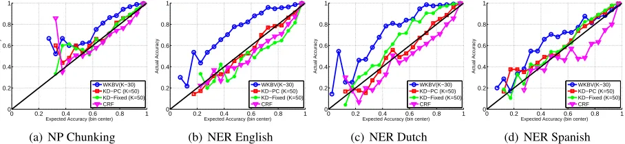
Figure 4:Predicted error in each bin vs. the actual frequency of mistakes in each bin. Best performance is obtained by methods

close to the liney = x(black line) for four tasks. Four methods are compared: weightedK-Viterbi (WKBV),K-draws PC (KD-PC) andK-draws fixed covariance (KD-Fixed) and CRF.

two best performing among the CW based methods are KD-Fixed and KD-PC, where the former is bet-ter in three out of four datasets. When compared to CRF we see that in two cases CRF outperforms the K-Draws based methods and in the other two cases it performs equally. We found the relative suc-cess of KD-Fixed compared to KD-PC surprising, as KD-Fixed does not take into consideration the ac-tual uncertainty in the parameters learned by CW, and in fact replaced it with afixed value across all features. Since this method does not need to as-sume a confidence-based learning approach we re-peated the experiment, training a model with the passive-aggressive algorithm, rather than CW. All confidence estimation methods can be used except the KD-PC, which does take the confidence infor-mation into consideration. The results appear in the bottom-left panel of Fig. 2, and basically tell the same story, KD-Fixed outperform the margin based method (Delta), and the Viterbi based meth-ods (KBV, WKBV).

To better understand the behavior of the various methods we plot the total number of detected erro-neous words vs. the number of ranked words (first 5,000ranked words) in the top panels of Fig. 3. The bottom panels show the relative additional number of words each methods detects on top of the margin-based Delta method. Clearly, Fixed and KD-PC detect erroneous words better than the other CW based methods, finding about100more words than Delta (when ranking 5,000 words) which is about 8%of the total number of erroneous words.

Regarding CRF, it outperforms the K-Draws methods in NER English and NP chunking datasets, finding about 150 more words, CRF performed equally for NER Dutch, and performed worse for

NER Spanish finding about80 less words. We em-phasize that all methodsexcept CRFwere based on the same exact weight vector, ranking the same pre-dations, while CRF used an alternative weight vector that yields different number of erroneous words.

In details, we observe some correlation between the percentage or erroneous words in the entire set and the number of erroneous words detected among the first 5,000 ranked words. For NP chunking and NER English datasets, CRF has more erroneous words compared to CW and it detects more erro-neous words compared to K-Draws. For NER Dutch dataset CRF and CW have almost same number of erroneous words and almost same number of erro-neous words detected, and finally in NER Spanish dataset CRF has fewer erroneous words and it de-tected less erroneous words. In other words, where there are more erroneous words to find (e.g. CRF in NP chunking), the task of ranking erroneous words is easier, and vice-versa.

We hypothesize that part of the performance dif-ferences we see between the K-Draws and CRF methods is due to the difference in the number of erroneous words in the ranked set.

This ranking view can be thought of marking sus-pected words to be evaluated manually by a human annotator. Although in general it may be hard for a human to annotate a single word with no need to an-notate its close neighbor, this is not the case here. As the neighbor words are already labeled, and pretty reliably, as mentioned above.

(9)

KBV, WKBV and CRF) were applied on the entire set of predicted labels. (Delta method is omitted as the confidence score it produces is not in[0,1]).

For each of the four datasets and the five algo-rithms we grouped the words according to the value of their confidence. Specifically, we used twenty (20) bins dividing uniformly the confidence range into intervals of size0.05. For each bin, we com-puted the fraction of words predicted correctly from the words assigned to that bin. Ultimately, the value of the computed frequency should be about the cen-ter value of the incen-terval of the bin. Formally, bin indexed j contains words with confidence value in the range[(j−1)/20, j/20)forj= 1. . .20. Letbj be the center value of binj, that isbj =j/20−1/40. The frequency of correct words in bin j, denoted by cj is the fraction of words with confidenceν ∈ [(j−1)/20, j/20)that their assigned label is correct. Ultimately, these two values should be the same, bj = cj, meaning that the confidence information is a good estimator of the frequency of correct la-bels. Methods for whichcj > bjare too pessimistic, predicting too high frequency of erroneous labels, while methods for whichcj < bjare too optimistic, predicting too low frequency of erroneous words.

The results are summarized in Fig 4, one panel per dataset, where we plot the value of the center-of-binbj vs. the frequency of correct predictioncj, connecting the points associated with a single algo-rithm. Four algorithms are shown: PC, KD-Fixed, WKBV and CRF. We omit the results of the KBV approach - they were substantially inferior to all other methods. Best performance is obtained when the resulting line is close to the liney=x.

From the plots we observe that WKBV is too pes-simistic as its corresponding line (blue square) is above the liney=x. CRF method is too optimistic, its corresponding line is below the line y = x. The KD-Fixed method is too pessimistic on NER-Dutch and too optimistic on NER-English. The best method is KD-PC which, surprisingly, tracks the line x =ypretty closely. We hypothesis that its superi-ority is because it makes use of the uncertainty infor-mation captured in the covariance matrixΣwhich is part of the Gaussian distribution.

Finally, these bins plots does not reflect the fact that different bins were not populated uniformly, the bins with higher values were more heavily

popu-lated. We thus plot in the top-right of Fig. 2 the root mean-square error in predicting the bin center

value given by r

P

jnj(bj−cj)2

/P jnj

,

where nj is the number of words in the jth bin. We observed a similar trend to the one appeared in the previous figure. WKBV is the least-performing method, then KD-Fixed and CRF, and then KD-PC which achieved lowest RMSE in all four datasets. Similar plot but when using PA for training appear in the bottom-right panel of Fig. 2. In this case we also see that KD-Fixed is better than WKBV, even though both methods were not trained with an algo-rithm that takes uncertainty information into consid-eration, like CW.

The success of KD-PC and KD-Fixed in evaluat-ing confidence led us to experiment with usevaluat-ing sim-ilar techniques for inference. Given an input sen-tence, the inference algorithm samplesKtimes from the Gaussian distribution and output the best label-ing accordlabel-ing to each sampled weight vector. Then the algorithm predicts for each word the most fre-quent label. We found this method inferior to infer-ence with the mean parameters. This approach dif-fers from the one used by (Crammer et al., 2009a), as they output the most frequent labeling in a set, while the predicted label of our algorithm may not even belong to the set of predictions.

6 Active Learning

Encouraged by the success of the PC and KD-Fixed algorithms in estimating the confidence in the prediction we apply these methods to the task of ac-tive learning. In acac-tive learning, the algorithm is given a large set of unlabeled data and a small set of labeled data and works in iterations. On each it-eration, the overall labeled data at this point is used to build a model, which is then used to choose new subset of examples to be annotated.

(10)

then used to choose new examples to be labeled. In our case the goal is to label sentences, which are expensive to label. We thus applied the following setting. First, we chose a subset of 9K sentences as unlabeled training set, and another subset of size 3K for evaluation. After obtaining a model, the al-gorithm labels random1,000sentences and chose a subset of10sentences using the active learning rule, which we will define shortly. After repeating this process10times we then evaluate the current model using the test data and proceed to choose new un-labeled examples to be un-labeled. Each method was applied to pick5,000sentences to be labeled.

In the previous section, we used the confidence estimation algorithms to choose individualwordsto be annotated by a human. This setting is realistic since most words in each sentence were already clas-sified (correctly). However, when moving to active learning, the situation changes. Now, all the words in a sentence are not labeled, thus a human may need to label additional words than the one in target, in or-der to label the target word. We thus experimented with the following protocol. On each iteration, the algorithm defines the score of an entire sentence to be the score of the least confident word in the sen-tence. Then the algorithm chooses the least confi-dent sentence, breaking ties by favoring shorter sen-tences (assuming they contain relatively more infor-mative words to be labeled than long sentences).

We evaluated five methods, PC and KD-Fixed mentioned above. The method that ranks a sentence by the difference in score between the top- and second-best labeling, averaged over the length of sentence, denoted by MinMargin (Tong and Koller, 2001). A similar approach, motivated by (Dredze and Crammer, 2008), normalizes Min-Margin score using the confidence information ex-tracted from the Gaussian covariance matrix, we call this method MinConfMargin. Finally, We also eval-uated an approach that picks random sentences to be labeled, denoted by RandAvg (averaged5times).

The averaged cumulative F-measure vs. num-ber of words labeled is presented in Figs. 5,6. We can see that for short horizon (small number of sen-tences) the MinMargin is worse (in three out of four data sets), while MinConfMargin is worse in NP Chunking. Then there is no clear winner, but the KD-Fixed seems to be the best most of the time. The

2000 4000 6000 8000 10000 0.84

0.85 0.86 0.87 0.88 0.89 0.9

Total No. of Labeled Words

F−Measure

KD−PC (50) KD−Fixed (K=50) MinMargin MinConfMargin RandAvg

(a) NP Chunking

2000 4000 6000 8000 10000 0.35

0.4 0.45 0.5 0.55 0.6

F−Measure

(b) NER English

104

0.9 0.905 0.91 0.915 0.92 0.925 0.93

F−Measure

(c) NP Chunking

104 0.62 0.64 0.66 0.68 0.7 0.72 0.74 0.76

F−Measure

[image:10.612.318.535.56.267.2]

(d) NER English

Figure 5: Averaged cumulative F-score vs. total number of

words labeled. The top panels show the results for up to10,000 labeled words, while the bottom panels show the results for more than10klabeled words.

bottom panels show the results for more than 10k training words. Here, the random method perform-ing the worst, while KD-PC and KD-Fixed are the best, and as shown in (Dredze and Crammer, 2008), MinConfMargin outperforming MinMargin.

Related Work: Most previous work has fo-cused on confidence estimation for an entire exam-ple or some fields of an entry (Culotta and McCal-lum, 2004) using CRFs. (Kristjansson et al., 2004) show the utility of confidence estimation is extracted fields of an interactive information extraction system by high-lighting low confidence fields for the user. (Scheffer et al., 2001) estimate confidence of sin-gle token label in HMM based information extrac-tion system by a method similar to the Delta method we used. (Ueffing and Ney, 2007) propose several methods for word level confidence estimation for the task of machine translation. One of the methods they use is very similar to the weighted and non-weighted K-best Viterbi methods we used with the proper ad-justments to the machine translation task.

Acknowledgments

(11)

2000 4000 6000 8000 10000 0.3

0.35 0.4 0.45 0.5 0.55

F−Measure

(a) NER Dutch

2000 4000 6000 8000 10000 0.32

0.34 0.36 0.38 0.4 0.42 0.44 0.46 0.48

F−Measure

(b) NER Spanish

104

0.58 0.6 0.62 0.64 0.66 0.68 0.7 0.72

F−Measure

(c) NER Dutch

104

105

0.48 0.5 0.52 0.54 0.56 0.58 0.6 0.62 0.64

F−Measure

[image:11.612.76.294.58.269.2]

(d) NER Spanish

Figure 6: See Fig. 5

References

[Cesa-Bianchi and Lugosi2006] N. Cesa-Bianchi and

G. Lugosi. 2006. Prediction, Learning, and Games.

Cambridge University Press, New York, NY, USA. [Collins2002] M. Collins. 2002. Discriminative training

methods for hidden markov models: Theory and

ex-periments with perceptron algorithms. InEMNLP.

[Crammer et al.2005] K. Crammer, R. Mcdonald, and F. Pereira. 2005. Scalable large-margin online learn-ing for structured classification. Tech. report, Dept. of CIS, U. of Penn.

[Crammer et al.2008] K. Crammer, M. Dredze, and

F. Pereira. 2008. Exact confidence-weighted learning. InNIPS 22.

[Crammer et al.2009a] K. Crammer, M. Dredze, and A. Kulesza. 2009a. Multi-class confidence weighted

algorithms. InEMNLP.

[Crammer et al.2009b] K. Crammer, A. Kulesza, and

M. Dredze. 2009b. Adaptive regularization of

weighted vectors. InNIPS 23.

[Culotta and McCallum2004] A. Culotta and A. McCal-lum. 2004. Confidence estimation for information

ex-traction. InHLT-NAACL, pages 109–112.

[Dredze and Crammer2008] M. Dredze and K. Crammer.

2008. Active learning with confidence. InACL.

[Dredze et al.2008] M. Dredze, K. Crammer, and

F. Pereira. 2008. Confidence-weighted linear

classification. InICML.

[Kim et al.2000] E.F. Tjong Kim, S. Buchholz, and K. Sang. 2000. Introduction to the conll-2000 shared task: Chunking.

[Kristjansson et al.2004] T. Kristjansson, A. Culotta,

P. Viola, and A. McCallum. 2004. Interactive infor-mation extraction with constrained conditional random

fields. InAAAI, pages 412–418.

[Lafferty et al.2001] J. Lafferty, A. McCallum, and

F. Pereira. 2001. Conditional random fields: Proba-bilistic models for segmenting and labeling sequence data.

[McCallum2002] Andrew McCallum. 2002. MALLET:

A machine learning for language toolkit. http://

mallet.cs.umass.edu.

[McDonald et al.2005a] R.T. McDonald, K. Crammer, and F. Pereira. 2005a. Flexible text segmentation with

structured multilabel classification. InHLT/EMNLP.

[McDonald et al.2005b] Ryan T. McDonald, Koby Cram-mer, and Fernando C. N. Pereira. 2005b. Online

large-margin training of dependency parsers. InACL.

[Scheffer et al.2001] Tobias Scheffer, Christian

Deco-main, and Stefan Wrobel. 2001. Active hidden

markov models for information extraction. In IDA,

pages 309–318, London, UK. Springer-Verlag. [Sha and Pereira2003] Fei Sha and Fernando Pereira.

2003. Shallow parsing with conditional random fields. InProc. of HLT-NAACL, pages 213–220.

[Shimizu and Haas2006] N. Shimizu and A. Haas. 2006. Exact decoding for jointly labeling and chunking

se-quences. InCOLING/ACL, pages 763–770.

[Taskar et al.2003] B. Taskar, C. Guestrin, and D. Koller.

2003. Max-margin markov networks. Innips.

[Tjong and Sang2002] Erik F. Tjong and K. Sang. 2002. Introduction to the conll-2002 shared task:

Language-independent named entity recognition. InCoNLL.

[Tjong et al.2003] E.F. Tjong, K. Sang, and F. De Meul-der. 2003. Introduction to the conll-2003 shared task: Language-independent named entity recognition. In

CoNLL, pages 142–147.

[Tong and Koller2001] S. Tong and D. Koller. 2001.

Support vector machine active learning with

applica-tions to text classification. InJMLR, pages 999–1006.

[Ueffing and Ney2007] Nicola Ueffing and Hermann Ney. 2007. Word-level confidence estimation for machine

translation.Comput. Linguist., 33(1):9–40.

[Wick et al.2009] M. Wick, K. Rohanimanesh, A. Cu-lotta, and A. McCallum. 2009. Samplerank: Learning

preferences from atomic gradients. InNIPS Workshop