Better Synchronous Binarization for Machine Translation

Better Synchronous Binarization for Machine Translation

Tong Xiao

, Mu Li

, Dongdong Zhang

, Jingbo Zhu

, Ming Zhou

*

Natural Language Processing Lab

Northeastern University

Shenyang, China, 110004

[email protected]

[email protected]

+

Microsoft Research Asia

Sigma Center

Beijing, China, 100080

[email protected]

[email protected]

[email protected]

Abstract

Binarization of Synchronous Context Free Grammars (SCFG) is essential for achieving polynomial time complexity of decoding for SCFG parsing based machine translation sys-tems. In this paper, we first investigate the excess edge competition issue caused by a left-heavy binary SCFG derived with the method of Zhang et al. (2006). Then we propose a new binarization method to mitigate the problem by exploring other alternative equivalent bi-nary SCFGs. We present an algorithm that ite-ratively improves the resulting binary SCFG, and empirically show that our method can im-prove a string-to-tree statistical machine trans-lations system based on the synchronous bina-rization method in Zhang et al. (2006) on the NIST machine translation evaluation tasks.

1

Introduction

Recently Statistical Machine Translation (SMT) systems based on Synchronous Context Free Grammar (SCFG) have been extensively investi-gated (Chiang, 2005; Galley et al., 2004; Galley et al., 2006) and have achieved state-of-the-art performance. In these systems, machine transla-tion decoding is cast as a synchronous parsing task. Because general SCFG parsing is an NP-hard problem (Satta and Peserico, 2005), practic-al SMT decoders based on SCFG parsing re-quires an equivalent binary SCFG that is directly learned from training data to achieve polynomial time complexity using the CKY algorithm (Ka-sami, 1965; Younger, 1967) borrowed from CFG parsing techniques. Zhang et al. (2006) proposed synchronous binarization, a principled method to

binarize an SCFG in such a way that both the source-side and target-side virtual non-terminals have contiguous spans. This property of syn-chronous binarization guarantees the polynomial time complexity of SCFG parsers even when an n-gram language model is integrated, which has been proved to be one of the keys to the success of a string-to-tree syntax-based SMT system.

However, as shown by Chiang (2007), SCFG-based decoding with an integrated n-gram lan-guage model still has a time complexity of 𝛩(𝑚3 _𝑇 4(𝑛−1)_{), where m is the source sentence} length, and 𝑇 is the vocabulary size of the lan-guage model. Although it is not exponential in theory, the actual complexity can still be very high in practice. Here is an example extracted from real data. Given the following SCFG rule:

VP → VB NP 会 JJR , VB NP will be JJR

we can obtain a set of equivalent binary rules using the synchronous binarization method (Zhang et al., 2006) as follows:

VP → V1 JJR , V1 JJR

V1 → VB V2 , VB V2

V2 → NP会 , NP will be

This binarization is shown with the solid lines as binarization (a) in Figure 1. We can see that bi-narization (a) requires that “NP 会” should be reduced at first. Data analysis shows that “NP 会” is a frequent pattern in the training corpus, and there are 874 binary rules of which the source language sides are “NP 会”. Consequently these binary rules generate a large number of compet-ing edges in the chart when “NP 会” is matched in decoding. To reduce the number of edges

posed in decoding, hypothesis re-combination is used to combine the equivalent edges in terms of dynamic programming. Generally, two edges can be re-combined if they satisfy the following two constraints: 1) the LHS (left-hand side) non-terminals are identical and the sub-alignments are the same (Zhang et al., 2006); and 2) the boundary words1 on both sides of the partial translations are equal between the two edges (Chiang, 2007). However, as shown in Figure 2, the decoder still generates 801 edges after the hypothesis re-combination. As a result, aggres-sive pruning with beam search has to be em-ployed to reduce the search space to make the decoding practical. Usually in beam search only a very small number of edges are kept in the beam of each chart cell (e.g. less than 100). These edges have to compete with each other to survive from the pruning. Obviously, more com-peting edges proposed during decoding can lead to a higher risk of making search errors.

VB NP 会 JJR

(a) (b)

V2 V1

V2' V1' VP

VB NP will be JJR

Figure 1: Two different binarizations (a) and (b) of the same SCFG rule distinguished by the

solid lines and dashed lines

我们 希望 情况 会 更好 。 (We hope the situation will be better .)

我们 希望 NP 会 JJR 。

decoding

match 874 rules match 62 rules

competing edges: 801 competing edges: 57

Figure 2: Edge competitions caused by different binarizations

The edge competition problem for SMT de-coding is not addressed in previous work (Zhang et al., 2006; Huang, 2007) in which each SCFG rule is binarized in a fixed way. Actually the re-sults of synchronous binarization may not be the only solution. As illustrated in Figure 1, the rule

1

For the case of n-gram language model integration,

2 × (𝑛 − 1) boundary words needs to be examined.

can also be binarized as binarization (b) which is shown with the dashed lines.

We think that this problem can be alleviated by choosing better binarizations for SMT decod-ers, since there is generally more than one bina-rization for a SCFG rule. In our investigation, about 96% rules that need to be binarized have more than one binarization under the contiguous constraint. As shown in binarization (b) (Figure 1), “会 JJR” is reduced first. In the decoder, the number of binary rules with the source-side “会

JJR” is 62, and the corresponding number of edges is 57 (Figure 2). The two numbers are both much smaller than those of “NP 会” in (a). This is an informative clue that the binarization (b) could be better than the binarization (a) based on the following: the probability of pruning the rule in (a) is higher than that in (b) as the rule in (b) has fewer competitors and has more chances to survive during pruning.

In this paper we propose a novel binarization method, aiming to find better binarizations to improve an SCFG-based machine translation system. We formulate the binarization optimiza-tion as a cost reducoptimiza-tion process, where the cost is defined as the number of rules sharing a common source-side derivation in an SCFG. We present an algorithm, iterative cost reduction algorithm, to obtain better binarization for the SCFG learnt automatically from the training corpus. It can work with an efficient CKY-style binarizer to search for the lowest-cost binarization. We apply our method into a state-of-the-art string-to-tree SMT system. The experimental results show that our method outperforms the synchronous binari-zation method (Zhang et al., 2006) with over 0.8 BLEU scores on both NIST 2005 and NIST 2008 Chinese-to-English evaluation data sets.

2

Related Work

The problem of binarization originates from the parsing problem in which several binarization methods are studied such as left/right binariza-tion (Charniak et al., 1998; Tsuruoka and Tsujii, 2004) and head binarization (Charniak et al., 2006). Generally, the pruning issue in SMT de-coding is unnecessary for the parsing problem, and the accuracy of parsing does not rely on the binarization method heavily. Thus, many efforts on the binarization in parsing are made for the efficiency improvement instead of the accuracy improvement (Song et al., 2008).

binarization method is proposed in (Zhang et al., 2006) whose basic idea is to build a left-heavy binary synchronous tree (Shapiro and Stephens, 1991) with a left-to-right shift-reduce algorithm. Target-side binarization is another binarization method which is proposed by Huang (2007). It works in a left-to-right way on the target lan-guage side. Although this method is compara-tively easy to be implemented, it just achieves the same performance as the synchronous binari-zation method (Zhang et al., 2006) for syntax-based SMT systems. In addition, it cannot be easily integrated into the decoding of some syn-tax-based models (Galley et al., 2004; Marcu et al., 2006), because it does not guarantee conti-guous spans on the source language side.

3

Synchronous Binarization

Optimiza-tion by Cost ReducOptimiza-tion

As discussed in Section 1, binarizing an SCFG in a fixed (left-heavy) way (Zhang et al., 2006) may lead to a large number of competing edges and consequently high risk of making search errors. Fortunately, in most cases a binarizable SCFG can be binarized in different ways, which pro-vides us with an opportunity to find a better solu-tion than the default left-heavy binarizasolu-tion. An ideal solution to this problem could be that we define an exact edge competition estimation function and choose the best binary SCFG based on it. However, even for the rules with a com-mon source-side, generally it is difficult to esti-mate the exact number of competing edges in the dynamic SCFG parsing process for machine translation, because in order to integrate an n -gram language model, the actual number of edges not only depends on SCFG rules, but also depends on language model states which are spe-cific to input sentences. Instead, we have to em-ploy certain kinds of approximation of it. First we will introduce some notations frequently used in later discussions.

3.1 Notations

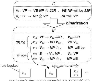
We use 𝐺 = {𝑅𝑖 ∶ 𝑋𝑖 → 𝛼𝑖, 𝛽𝑖} to denote an SCFG, where 𝑅𝑖 is the 𝑖𝑡ℎ rule in 𝐺; 𝑋𝑖 is the LHS (left hand side) non-terminal of 𝑅𝑖; 𝛼𝑖 and 𝛽_𝑖 are the source-side and target-side RHS (right hand side) derivations of 𝑅𝑖 respectively. We use ℬ 𝐺 to denote the set of equivalent binary SCFG of 𝐺. The goal of SCFG binarization is to find an appropriate binary SCFG 𝐺′ ∈ ℬ 𝐺 . For 𝑅_𝑖 , ℬ 𝑅_𝑖 = {𝑣_𝑖𝑗} ⊆ 𝐺′ ∈ ℬ 𝐺 is the set of equivalent binary rules based on 𝑅𝑖, where 𝑣𝑖𝑗 is

the 𝑗𝑡ℎ binary rule in ℬ 𝑅𝑖 . Figure 3 illustrates the meanings of these notations with a sample grammar.

VP→ VBNP会JJR , VBNP will be JJR S → NP会VP , NP will VP

R1 :

R2 :

G

VP → V12JJR , V12JJR (R1)

G’

V12→VBV13 , VBV13

V13→ NP会 , NP will be v11 :

v12 :

v13 :

S → V22VP , V22VP

V22→NP会 , NPwill v21 :

v22 :

(R2)

binarization

...

v11 v12 v22

S(“VB NP 会 JJR ”, G’) S(“VB NP 会”, G’) S(“NP 会”, G’) L(v12)=”VB NP 会”

v13 rule bucket

Figure 3: Binarization on a sample grammar

The function 𝐿(∙) is defined to map a result-ing binary rule 𝑣𝑖𝑗𝜖𝐺′ to the sub-sequence in 𝛼𝑖 derived from 𝑣_𝑖𝑗. For example, as shown in Fig-ure 3, the binary rule 𝑣₁₃ covers the source sub-sequence “NP 会” in 𝑅₁, so 𝐿 𝑣13 = "NP 会". Similarly, 𝐿 𝑣₁₂ = "VB NP 会".

The function 𝐿(∙) is used to group the rules in 𝐺′ with a common right-hand side derivation for source language. Given a binary rule 𝑣 ∈ 𝐺′, we can put it into a bucket in which all the binary rules have the same source sub-sequence 𝐿(𝑣). For example (Figure 3), as 𝐿 𝑣12 = "VB NP 会", 𝑣₁₂ is put into the bucket indexed by “VB NP 会”. And 𝑣₁₃ and 𝑣₂₂ are put into the same bucket, since they have the same source sub-sequence “NP 会”. Obviously, 𝐺′ can be divided into a set of mutual exclusive rule buckets by 𝐿(∙).

In this paper, we use 𝑆(𝐿(𝑣), 𝐺′) to denote the bucket for the binary rules having the source sub-sequence 𝐿(𝑣). For example, 𝑆("𝑁𝑃 会", 𝐺′) de-notes the bucket for the binary rules having the source-side “NP 会”. For simplicity, we also use 𝑆(𝑣, 𝐺′) to denote 𝑆 𝐿 𝑣 , 𝐺′ .

3.2 Cost Reduction for SCFG Binarization

Each application of other rules in the bucket 𝑆(𝑣, 𝐺′) can generate competing edges with the one based on 𝑣. Intuitively, the size of bucket can be used to approximately indicate the actual number of competing edges on average, and re-ducing the size of bucket could help reduce the edges generated in a parsing chart by applying the rules in the bucket. Therefore, if we can find a method to greedily reduce the size of each bucket 𝑆(𝑣, 𝐺′), we can reduce the overall ex-pected edge competitions when parsing with 𝐺′.

However, it can be easily proved that the numbers of binary rules in any 𝐺′ ∈ ℬ 𝐺 are same, which implies that we cannot reduce the sizes of all buckets at the same time – removing a rule from one bucket means adding it to anoth-er. Allowing for this fact, the excess edge com-petition example shown in Section 1 is essential-ly caused by the uneven distribution of rules among different buckets 𝑆 ∙ . Accordingly, our optimization objective should be a more even distribution of rules among buckets.

In the following, we formally define a metric to model the evenness of rule distribution over buckets. Given a binary SCFG 𝐺′ and a binary SCFG rule 𝑣 ∈ 𝐺′, 𝑄(𝑣) is defined as the cost function that maps 𝑣 to the size of the bucket 𝑆 𝑣, 𝐺′ :

𝑄 𝑣 = 𝑆 𝑣, 𝐺′ (1)

Obviously, all the binary rules in 𝑆 𝑣, 𝐺′ share a common cost value 𝑆 𝑣, 𝐺′ . For example (Fig-ure 3), both 𝑣13 and 𝑣22 are put into the same

bucket 𝑆 "𝑁𝑃 会", 𝐺′ , so 𝑄 𝑣13 = 𝑄 𝑣22 = 2.

The cost of the SCFG 𝐺′ is computed by summing up all the costs of SCFG rules in it:

𝑄 𝐺′ = 𝑄(𝑣)

𝑣∈𝐺′ (2)

Back to our task, we are to find an equivalent binary SCFG 𝐺′ of 𝐺 with the lowest cost in terms of the cost function 𝑄(. ) given in Equation (2):

𝐺∗_{= argmin}

𝐺′∈ℬ 𝐺 𝑄(𝐺′) (3)

Next we will show how 𝐺∗ is related to the evenness of rule distribution among different buckets. Let 𝑆 𝐺′ = {𝑆1, … , 𝑆𝑀} be the set of rule buckets containing rules in 𝐺′, then the value of 𝑄(𝐺′) can also be written as:

𝑄 𝐺′ = 𝑆𝑖 2

1≤𝑖≤𝑀 (4)

Assume 𝑌_𝑖 = 𝑆_𝑖 is an empirical distribution of a discrete random variable 𝑌, then the square devi-ation of the empirical distribution is:

𝜎2₌ 1

𝑀 ( 𝑆𝑖 𝑖 − 𝑌 )2 (5)

Noticing that Σ 𝑆𝑖 = 𝐺′ and 𝑌 = 𝐺′ /𝑀, Equ-ation (5) can be written as:

𝜎2 ₌ 1

𝑀 𝑄 𝐺′ − 𝐺′ 2

𝑀 (6)

Since both 𝑀 and |𝐺′| are constants, minimizing the cost function 𝑄(𝐺′) is equivalent to minimiz-ing the square deviation of the distribution of rules among different buckets. A binary SCFG with the lower cost indicates the rules are more evenly distributed in terms of derivation patterns on the source language side.

3.3 Static Cost Reduction

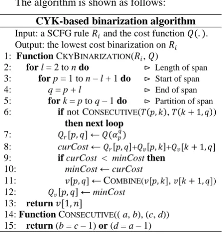
Before moving on discussing the algorithm which can optimize Equation (3) based on rule costs specified in Equation (1), we first present an algorithm to find the optimal solution to Eq-uation (3) if we have known the cost setting of 𝐺∗ _{and can use the costs as static values during} binarization. Using this simplification, the prob-lem of finding the binary SCFG 𝐺∗ with minim-al costs can be reduced to find the optimminim-al bina-rization ℬ∗(𝑅_𝑖) for each rule 𝑅_𝑖 in 𝐺.

To obtain ℬ∗(𝑅𝑖), we can employ a CKY-style binarization algorithm which builds a com-pact binarization forest for the rule 𝑅𝑖 in bottom-up direction. The algorithm combines two adja-cent spans of 𝛼_𝑖 each time, in which two spans can be combined if and only if they observe the BTG constraints−their translations are either sequentially or reversely adjacent in 𝛽𝑖, the tar-get-side derivation of 𝑅_𝑖. The key idea of this algorithm is that we only use the binarization tree with the lowest cost of each span for later com-bination, which can avoid enumerating all the possible binarization trees of 𝑅𝑖 using dynamic programming.

Let 𝛼_𝑝𝑞 be the sub-sequence spanning from p to q on the source-side, 𝑣[𝑝, 𝑞] be optimal bina-rization tree spanning 𝛼_𝑝𝑞, 𝑄𝑣[𝑝, 𝑞] be the cost of 𝑣[𝑝, 𝑞], and 𝑄𝑟[𝑝, 𝑞] be the cost of any binary rules whose source-side is 𝛼_𝑝𝑞, then the cost of optimal binarization tree spanning 𝛼_𝑝𝑞 can be computed as:

The algorithm is shown as follows:

CYK-based binarization algorithm

Input: a SCFG rule 𝑅_𝑖 and the cost function 𝑄(. ). Output: the lowest cost binarization on 𝑅𝑖

1: Function CKYBINARIZATION(𝑅_𝑖, 𝑄)

2: for l = 2 to n do ⊳ Length of span

3: for p = 1 to n – l +1 do ⊳ Start of span

4: q = p + l ⊳ End of span

5: for k = p to q – 1 do ⊳ Partition of span 6: if not CONSECUTIVE(𝑇 𝑝, 𝑘 , 𝑇 𝑘 + 1, 𝑞 ) then next loop

7: 𝑄𝑟[𝑝, 𝑞] ← 𝑄(𝛼𝑝𝑞)

8: curCost ← 𝑄𝑟 𝑝, 𝑞 +𝑄𝑣 𝑝, 𝑘 +𝑄𝑣[𝑘 + 1, 𝑞]

9: if curCost < minCost then 10: minCost ← curCost

11: 𝑣[𝑝, 𝑞]←COMBINE(𝑣[𝑝, 𝑘], 𝑣[𝑘 + 1, 𝑞])

12: 𝑄𝑣 𝑝, 𝑞 ← minCost

13: return 𝑣[1, 𝑛]

14: Function CONSECUTIVE(( a, b), (c, d)) 15: return (b = c – 1) or (d = a – 1)

where n is the number of tokens (consecutive terminals are viewed as a single token) on the source-side of 𝑅𝑖. COMBINE(𝑣[𝑝, 𝑘], 𝑣[𝑘 + 1, 𝑞])

combines the two binary sub-trees into a larger sub-tree over 𝛼_𝑝𝑞. 𝑇 𝑝, 𝑞 = (𝑎, 𝑏) means that the non-terminals covering 𝛼_𝑝𝑞 have the consecutive indices ranging from a to b on the target-side. If the target non-terminal indices are not consecu-tive, we set 𝑇 𝑝, 𝑞 = (−1, −1). 𝑄 𝛼_𝑝𝑞 = 𝑄(𝑣′) where 𝑣′ is any rule in the bucket 𝑆 𝛼𝑝𝑞, 𝐺′ .

In the algorithm, lines 9-11 implement dynam-ic programming, and the function CONSECUTIVE

checks whether the two spans can be combined.

VB NP 会

V[1,2] V[3,4]

VP

JJR V[2,3]

V[1,3] V[2,4]

c=6619 c=874 c=62 c=884 c=876 c=64 c=6629

c=885 c=6682 c=65

VB NP will be JJR lowest cost

c=0 c=0 c=0 c=0

Figure 4: Binarization forest for an SCFG rule

𝐿(𝑣) 𝑄(𝑣) 𝐿(𝑣) 𝑄(𝑣)

VB NP 6619 VB NP 会 10

NP 会 874 NP 会 JJR 2

会 JJR 62 VB NP 会 JJR 1

Table 1: Sub-sequences and corresponding costs

Figure 4 shows an example of the compact forest the algorithm builds, where the solid lines indicate the optimal binarization of the rule, while other alternatives pruned by dynamic pro-gramming are shown in dashed lines. The costs

for binarization trees are computed based on the cost table given in Table 1.

The time complexity of the CKY-based bina-rization algorithm is Θ(n3), which is higher than that of the linear binarization such as the syn-chronous binarization (Zhang et al., 2006). But it is still efficient enough in practice, as there are generally only a few tokens (n < 5) on the source-sides of SCFG rules. In our experiments, the linear binarization method is just 2 times faster than the CKY-based binarization.

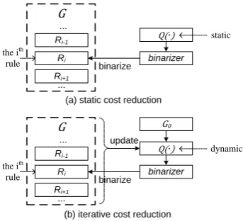
3.4 Iterative Cost Reduction

However, 𝑄(∙) cannot be easily predetermined in a static way as is assumed in Section 3.3 because it depends on 𝐺′ and should be updated whenever a rule in 𝐺 is binarized differently. In our work this problem is solved using the iterative cost reduction algorithm, in which the update of 𝐺′ and the cost function 𝑄(∙) are coupled together.

Iterative cost reduction algorithm

Input: An SCFG 𝐺

Output: An equivalent binary SCFG 𝐺′ of 𝐺 1: Function ITERATIVECOSTREDUCTION(𝐺) 2: 𝐺′← 𝐺0

3: for each 𝑣 ∈ 𝐺0do 4: 𝑄(𝑣) = 𝑆 𝑣, 𝐺0

5: while 𝑄(𝐺′)does not converge do 6: for each 𝑅𝑖 ∈ 𝐺 do

7: 𝐺[−𝑅_𝑖] ← 𝐺′ − ℬ(𝑅𝑖) 8: for each 𝑣 ∈ℬ(𝑅_𝑖) do 9: for each 𝑣′ ∈𝑆 𝑣, 𝐺′ do 10: 𝑄 𝑣′ ← 𝑄 𝑣′ − 1

11: ℬ(𝑅_𝑖) ← CKYBINARIZATION(𝑅_𝑖, 𝑄) 12: 𝐺′← 𝐺[−𝑅_𝑖]∪ ℬ(𝑅𝑖)

13: for each 𝑣 ∈ℬ(𝑅𝑖) do 14: for each 𝑣′ ∈𝑆 𝑣, 𝐺′ do 15: 𝑄 𝑣′ ← 𝑄 𝑣′ + 1 16: return 𝐺′

In the iterative cost reduction algorithm, we first obtain an initial binary SCFG 𝐺0 using the synchronous binarization method proposed in (Zhang et al., 2006). Then 𝐺₀ is assigned to an iterative variable 𝐺′. The cost of each binary rule in 𝐺0 is computed based on 𝐺0 according to Equ-ation (1) (lines 3-4 in the algorithm).

im-plement the cost reduction of each binary rule in the bucket 𝑆 𝑣, 𝐺′ .

Next, we find the lowest cost binarization for 𝑅_𝑖 based on the updated cost function 𝑄(∙) with the CKY-based binarization algorithm presented in Section 3.3 (line 11).

At last, the new binarization for 𝑅𝑖 is added back to 𝐺′ and 𝑄(∙) is re-updated to synchronize with this change (lines 12-15). Figure 5 illu-strates the differences between the static cost reduction and the iterative cost reduction.

Ri

Ri-1

Ri+1

...

...

the ith

rule G

binarizer Q(∙)

binarize

(a) static cost reduction

Ri

Ri-1

Ri+1

...

...

the ith

rule G

binarizer Q(∙)

G0

(b) iterative cost reduction update

static

dynamic

binarize

Figure 5: Comparison between the static cost reduction and the iterative cost reduction

The algorithm stops when 𝑄(𝐺′) does not de-crease any more. Next we will show that 𝑄(𝐺′) is guaranteed not to increase in the iterative process.

For any ℬ(𝑅𝑖)on 𝑅𝑖, we have

𝑄 𝐺_{[−𝑅𝑖]}∪ ℬ 𝑅_𝑖

= 2 × 𝑄 ℬ 𝑅𝑖 + ℬ 𝑅𝑖 + 𝑄 𝐺[−𝑅𝑖]

As both ℬ 𝑅𝑖 and 𝑄 𝐺[−𝑅𝑖] are constants with

respect to 𝑄(ℬ 𝑅_𝑖 ), 𝑄 𝐺[−𝑅_𝑖]∪ ℬ 𝑅𝑖 is a

li-near function of 𝑄(ℬ 𝑅_𝑖 ), and the correspond-ing slope is positive. Thus 𝑄 𝐺[−𝑅𝑖]∪ ℬ 𝑅𝑖 reaches the lowest value only when 𝑄(ℬ 𝑅𝑖 ) reaches the lowest value. So 𝑄 𝐺[−𝑅_𝑖]∪ ℬ 𝑅𝑖

achieves the lowest cost when we replace the current binarization with the new binarization ℬ∗_(𝑅

𝑖) (line 12). Therefore 𝑄 𝐺[−𝑅_𝑖]∪ ℬ 𝑅𝑖

does not increase in the processing on each 𝑅𝑖 (lines 7-15), and 𝑄(𝐺′) will finally converge to a local minimum when the algorithm stops.

4

Experiments

The experiments are conducted on Chinese-to-English translation in a state-of-the-art

string-to-tree SMT system. All the results are reported in terms of case-insensitive BLEU4(%).

4.1 Experimental Setup

Our bilingual training corpus consists of about 350K bilingual sentences (9M Chinese words + 10M English words)2. Giza++ is employed to perform word alignment on the bilingual sen-tences. The parse trees on the English side are generated using the Berkeley Parser3. A 5-gram language model is trained on the English part of LDC bilingual training data and the Xinhua part of Gigaword corpus. Our development data set comes from NIST2003 evaluation data in which the sentences of more than 20 words are ex-cluded to speed up the Minimum Error Rate Training (MERT). The test data sets are the NIST evaluation sets of 2005 and 2008.

Our string-to-tree SMT system is built based on the work of (Galley et al., 2006; Marcu et al., 2006), where both the minimal GHKM and SPMT rules are extracted from the training cor-pus, and the composed rules are generated by combining two or three minimal GHKM and SPMT rules. Before the rule extraction, we also binarize the parse trees on the English side using Wang et al. (2007) „s method to increase the coverage of GHKM and SPMT rules. There are totally 4.26M rules after the low frequency rules are filtered out. The pruning strategy is similar to the cube pruning described in (Chiang, 2007). To achieve acceptable translation speed, the beam size is set to 50 by default. The baseline system is based on the synchronous binarization (Zhang et al., 2006).

4.2 Binarization Schemes

Besides the baseline (Zhang et al., 2006) and iterative cost reduction binarization methods, we also perform right-heavy and random synchron-ous binarizations for comparison. In this paper, the random synchronous binarization is obtained by: 1) performing the CKY binarization to build the binarization forest for an SCFG rule; then 2) performing a top-down traversal of the forest. In the traversal, we randomly pick a feasible binari-zation for each span, and then go on the traversal in the two branches of the picked binarization.

Table 2 shows the costs of resulting binary SCFGs generated using different binarization methods. The costs of the baseline (left-heavy)

2 _{LDC2003E14, LDC2003E07, LDC2005T06 and}

LDC2005T10 3

and right-heavy binarization are similar, while the cost of the random synchronous binarization is lower than that of the baseline method4. As expected, the iterative cost reduction method ob-tains the lowest cost, which is much lower than that of the other three methods.

Method cost of binary SCFG 𝐺′

Baseline 4,897M

Right-heavy 5,182M

Random 3,479M

Iterative cost reduction 185M

Table 2: Costs of the binary SCFGs generated using different binarization methods.

4.3 Evaluation of Translations

Table 3 shows the performance of SMT systems based on different binarization methods. The iterative cost reduction binarization method achieves the best performance on the test sets as well as the development set. Compared with the baseline method, it obtains gains of 0.82 and 0.84 BLEU scores on NIST05 and NIST08 test sets respectively. Using the statistical signific-ance test described by Koehn (2004), the im-provements are significant (p < 0.05).

Method Dev NIST05 NIST08

Baseline 40.02 37.90 27.53

Right-heavy 40.05 37.87 27.40

Random 40.10 37.99 27.58

Iterative cost reduction

40.97* 38.72* 28.37*

Table 3: Performance (BLUE4(%)) of different binarization methods. * = significantly better than baseline (p < 0.05).

The baseline method and the right-heavy bina-rization method achieve similar performance, while the random synchronous binarization me-thod performs slightly better than the baseline method, which agrees with the fact of the cost reduction shown in Table 2. A possible reason that the random synchronous binarization me-thod can outperform the baseline meme-thod lies in that compared with binarizing SCFG in a fixed way, the random synchronous binarization tends to give a more even distribution of rules among buckets, which alleviates the problem of edge competition. However, since the high-frequency source sub-sequences still have high probabilities to be generated in the binarization and lead to the

4 _{We perform random synchronous binarization for 5} times and report the average cost.

excess competing edges, it just achieves a very small improvement.

4.4 Translation Accuracy vs. Cost of Binary

SCFG

We also study the impacts of cost reduction on translation accuracy over iterations in iterative cost reduction. Figure 6 and Figure 7 show the results on NIST05 and NIST08 test sets. We can see that the cost of the resulting binary SCFG drops greatly as the iteration count increases, especially in the first iteration, and the BLEU scores increase as the cost decreases.

Figure 6: Cost of binary SCFG vs. BLEU4 (NIST05)

Figure 7: Cost of binary SCFG vs. BLEU4 (NIST08)

4.5 Impact of Beam Size

In this section, we study the impacts of beam sizes on translation accuracy as well as compet-ing edges. To explicitly investigate the issue un-der large beam sizes, we use a subset of NIST05 and NIST08 test sets for test, which has 50 Chi-nese sentences of no longer than 10 words.

Figure 8 shows that the iterative cost reduction method is consistently better than the baseline method under various beam settings. Besides the experiment on the test set of short sentences, we also conduct the experiment on NIST05 test set. To achieve acceptable decoding speed, we range the beam size from 10 to 70. As shown in Figure 9, the iterative cost reduction method also out-performs the baseline method under various beam settings on the large test set.

Though enlarging beam size can reduce the search errors and improve the system perfor-mance, the decoding speed of string-to-tree SMT drops dramatically when we enlarge the beam size. The problem is more serious when long

1.0E+08 1.0E+09 1.0E+10

37.8 38 38.2 38.4 38.6 38.8

0 1 2 3 4 5 performance(BLEU4) cost

iteration BLEU4(%) cost of G'

1.0E+08 1.0E+09 1.0E+10

27.4 27.6 27.8 28 28.2 28.4

0 1 2 3 4 5 performance(BLEU4) cost BLEU4(%) cost of G'

sentences are translated. For example, when the beam size is set to a larger number (e.g. 200), our decoder takes nearly one hour to translate a sen-tence whose length is about 20 on a 3GHz CPU. Decoding on the entire NIST05 and NIST08 test sets with large beam sizes is impractical.

Figure 8: BLEU4 against beam size (small test set)

Figure 9: BLEU4 against beam size (NIST05)

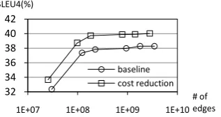
Figure 10 compares the baseline method and the iterative cost reduction method in terms of translation accuracy against the number of edges proposed during decoding. Actually, the number of edges proposed during decoding can be re-garded as a measure of the size of search space. We can see that the iterative cost reduction me-thod outperforms the baseline meme-thod under var-ious search effort.

Figure 10: BLEU4 against competing edges

The experimental results of this section show that compared with the baseline method, the iter-ative cost reduction method can lead to much fewer edges (about 25% reduction) as well as the higher BLEU scores under various beam settings.

4.6 Edge Competition vs. Cost of Binary

SCFG

In this section, we study the impacts of cost re-duction on the edge competition in the chart cells of our CKY-based decoder. Two metrics are

used to evaluate the degree of edge competition. They are the variance and the mean of the num-ber of competing edges in the chart cells, where high variance means that in some chart cells the rules have high risk to be pruned due to the large number of competing edges. The same situation holds for the mean as well. Both of the two me-trics are calculated on NIST05 test set, varying with the span length of chart cell.

Figure 11 shows the cost of resulting binary SCFG and the variance of competing edges against iteration count in iterative cost reduction. We can see that both the cost and the variance reduce greatly as the iteration count increases. Figure 12 shows the case for mean, where the reduction of cost also leads to the reduction of the mean value. The results shown in Figure 11 and Figure 12 indicate that the cost reduction is helpful to reduce edge competition in the chart cells.

Figure 11: Cost of binary SCFG vs. variance of competing edge number (NIST05)

Figure 12: Cost of binary SCFG vs. mean of competing edge number (NIST05)

We also perform decoding without pruning (i.e. beam size = ∞) on a very small set which has 20 sentences of no longer than 7 words. In this experiment, the baseline system and our iter-ative cost reduction based system propose 14,454M and 10,846M competing edges respec-tively. These numbers can be seen as the real numbers of the edges proposed during decoding instead of an approximate number observed in the pruned search space. It suggests that our me-thod can reduce the number of the edges in real search space effectively. A possible reason to

32 34 36 38 40 42

10 50 100 500 1000 5000

baseline cost reduction BLEU4(%)

beam size

35 36 37 38 39

10 20 30 40 50 70

baseline cost reduction

beam size

BLEU4(%)

32 34 36 38 40 42

1E+07 1E+08 1E+09 1E+10 baseline cost reduction BLEU4(%)

# of edges

1.0E+5 1.0E+6 1.0E+7 1.0E+8 1.0E+9 1.0E+10

1.0E+7 1.0E+8 1.0E+9 1.0E+10

0 1 2 3 4 5

span=2 span=3 span=5 span=7 span=10 span=20 cost

iteration variance cost of G'

1.0E+6 1.0E+7 1.0E+8 1.0E+9 1.0E+10

8.0E+3 1.0E+5

0 1 2 3 4 5

span=2 span=3 span=5 span=7 span=10 span=20 cost

this result is that the cost reduction based binari-zation could reduce the probability of rule mis-matching caused by binarization, which results in the reduction of the number of edges proposed during decoding.

5

Conclusion and Future Work

This paper introduces a new binarization method, aiming at choosing better binarization for SCFG-based SMT systems. We demonstrate the effec-tiveness of our method on a state-of-the-art string-to-tree SMT system. Experimental results show that our method can significantly outper-form the conventional synchronous binarization method, which indicates that better binarization selection is very beneficial to SCFG-based SMT systems.

In this paper the cost of a binary rule is de-fined based on the competition among the binary rules that have the same source-sides. However, some binary rules with different source-sides may also have competitions in a chart cell. We think that the cost of a binary rule can be better estimated by taking the rules with different source-sides into account. We intend to study this issue in our future work.

Acknowledgements

The authors would like to thank the anonymous reviewers for their pertinent comments, and Xi-nying Song, Nan Duan and Shasha Li for their valuable suggestions for improving this paper.

References

Eugene Charniak, Mark Johnson, Micha Elsner, Jo-seph Austerweil, David Ellis, Isaac Haxton, Cathe-rine Hill, R. Shrivaths, Jeremy Moore, Michael Po-zar, and Theresa Vu. 2006. Multilevel Coarse-to-Fine PCFG Parsing. In Proc. of HLT-NAACL 2006, New York, USA, 168-175.

Eugene Charniak, Sharon Goldwater, and Mark John-son. 1998. Edge-Based Best-First Chart Parsing. In

Proc. of the Six Workshop on Very Large Corpora, pages: 127-133.

David Chiang. 2005. A Hierarchical Phrase-Based Model for Statistical Machine Translation. In Proc. of ACL 2005, Ann Arbor, Michigan, pages: 263-270.

David Chiang. 2007. Hierarchical Phrase-based Translation. Computational Linguistics. 33(2): 202-208.

Michel Galley, Jonathan Graehl, Kevin Knight, Da-niel Marcu, Steve DeNeefe, Wei Wang, and

Igna-cio Thayer. 2006. Scalable Inference and Training of Context-Rich Syntactic Translation Models. In

Proc. of ACL 2006, Sydney, Australia, pages: 961-968.

Michel Galley, Mark Hopkins, Kevin Knight, and Daniel Marcu. 2004. What‟s in a translation rule? In Proc. of HLT-NAACL 2004, Boston, USA, pag-es: 273-280.

Liang Huang. 2007. Binarization, Synchronous Bina-rization, and Target-side binarization. In Proc. of HLT-NAACL 2007 / AMTA workshop on Syntax and Structure in Statistical Translation, New York, USA, pages: 33-40.

Tadao Kasami. 1965. An Efficient Recognition and Syntax Analysis Algorithm for Context-Free Lan-guages. Technical Report AFCRL-65-758, Air Force Cambridge Research Laboratory, Bedford, Massachusetts.

Philipp Koehn. 2004. Statistical Significance Tests for Machine Translation Evaluation. In Proc. of EMNLP 2004, Barcelona, Spain , pages: 388–395.

Daniel Marcu, Wei Wang, Abdessamad Echihabi, and Kevin Knight. 2006. SPMT: Statistical machine translation with syntactified target language phras-es. In Proc. of EMNLP 2006, Sydney, Australia, pages: 44-52.

Giorgio Satta and Enoch Peserico. 2005. Some Com-putational Complexity Results for Synchronous

Context-Free Grammars. In Proc. of HLT-EMNLP

2005, Vancouver, pages: 803-810.

L. Shapiro and A. B. Stephens. 1991. Bootstrap per-colation, the Sch𝑟 oder numbers, and the n-kings problem. SIAM Journal on Discrete Mathematics, 4(2):275-280.

Xinying Song, Shilin Ding and Chin-Yew Lin. 2008. Better Binarization for the CKY Parsing. In Proc. of EMNLP 2008, Hawaii, pages: 167-176.

Yoshimasa Tsuruoka and Junichi Tsujii. 2004. Itera-tive CKY Parsing for Probabilistic Context-Free Grammars. In Proc. of IJCNLP 2004, pages: 52-60.

Wei Wang and Kevin Knight and Daniel Marcu. 2007. Binarizing Syntax Trees to Improve Syntax-Based Machine Translation Accuracy. In Proc. of EMNLP-CoNLL 2007, Prague, Czech Republic, pages: 746-754.

D. H. Younger. 1967. Recognition and Parsing of Context-Free Languages in Time n3. Information and Control, 10(2):189-208.