Graphical Models over Multiple Strings
∗ Markus Dreyer and Jason EisnerDepartment of Computer Science / Johns Hopkins University Baltimore, MD 21218, USA
{markus,jason}@cs.jhu.edu
Abstract
We study graphical modeling in the case of
string-valued random variables. Whereas a weighted
finite-state transducer can model the probabilis-tic relationship betweentwostrings, we are inter-ested in building up joint models ofthree or more
strings. This is needed for inflectional paradigms
in morphology, cognate modeling or language re-construction, and multiple-string alignment. We propose a Markov Random Field in which each factor (potential function) is a weighted finite-state machine, typically a transducer that evaluates the relationship between just two of the strings. The full joint distribution is then a product of these fac-tors. Though decoding is actually undecidable in general, we can still do efficient joint inference using approximate belief propagation; the nec-essary computations and messages are all finite-state. We demonstrate the methods by jointly pre-dicting morphological forms.
1 Overview
This paper considers what happens if a graphical model’s variables can range over strings of un-bounded length, rather than over the typicalfinite
domains such as booleans, words, or tags. Vari-ables that are connected in the graphical model are related by some weighted finite-state transduction. Graphical models have become popular in ma-chine learning as a principled way to work with collections of interrelated random variables. Most often they are used as follows:
1. Build: Manually specify the n variables of interest; their domains; and the possible di-rect interactions among them.
2. Train: Train this model’s parameters θ to obtain a specific joint probability distribution
p(V1, . . . , Vn)over thenvariables.
3. Infer: Use this joint distribution to predict the values of various unobserved variables from observed ones.
∗Supported by the Human Language Technology Center
of Excellence at Johns Hopkins University, and by National Science Foundation grant No. 0347822 to the second author.
Note that 1. requires intuitions about the domain; 2. requires some choice of training procedure; and 3. requires a choice of exact or approximate infer-ence algorithm.
Our graphical models over strings are natural objects to investigate. We motivate them with some natural applications in computational lin-guistics (section 2). We then give our formalism: a Markov Random Field whose potential functions are rational weighted languages and relations (sec-tion 3). Next, we point out that inference is in gen-eral undecidable, and explain how to do approxi-mate inference using message-passing algorithms such as belief propagation (section 4). The mes-sages are represented as weighted finite-state ma-chines.
Finally, we report on some initial experiments using these methods (section 7). We use incom-plete data to train a joint model of morphological paradigms, then use the trained model to complete the data by predicting unseen forms.
2 Motivation
The problem of mapping between different forms and representations of strings is ubiquitous in nat-ural language processing and computational lin-guistics. This is typically done between string
pairs, where a pronunciation is mapped to its
spelling, an inflected form to its lemma, a spelling variant to its canonical spelling, or a name is transliterated from one alphabet into another. However, many problems involve more than just two strings:
• inmorphology, the inflected forms of a
(possi-bly irregular) verb are naturally considered to-gether as a whole morphological paradigm in which different forms reinforce one another;
• mapping an English word to its foreign
translit-eration may be easier when one considers the
orthographic and phonological forms of both words;
• similarcognatesin multiple languages are nat-urally described together, in orthographic or phonological representations, or both;
• modern and ancestral word forms form a phylo-genetic tree inhistorical linguistics;
• in bioinformatics and in system combination,
multiple sequences need to be aligned in order to identify regions of similarity.
We propose a unified model for multiple strings that is suitable for all the problems mentioned above. It is robust and configurable and can make use of task-specific overlapping features. It learns from observed and unobserved, or latent, in-formation, making it useful in supervised, semi-supervised, and unsupervised settings.
3 Formal Modeling Approach 3.1 Variables
AMarkov Random Field(MRF) is a joint model of a set of random variables, V = {V1, . . . , Vn}. We assume that all variables are string-valued, i.e. the value ofVi may be any string∈Σ∗i, whereΣi is some finite alphabet.
We may use meaningful names for the integers
i, such asV2SAfor the2ndsingular pastform of a verb.
The assumption that all variables are string-valued is not crucial; it merely simplifies our presentation. It is, however, sufficient for many practical purposes, since most other discrete ob-jects can be easily encoded as strings. For exam-ple, if V1 is a part of speech tag, it may be en-coded as a length-1 string over the finite alphabet
Σ1=def {Noun,Verb, . . .}.
3.2 Factors
A Markov Random Field defines a probability for each assignmentAof values to the variables inV:
p(A) =def 1
Z
m Y
j=1
Fj(A) (1)
This distribution over assignments is specified by the collection of factors Fj : A 7→ R≥0. Each factor (orpotential function) is a function that de-pends on only asubsetofA.
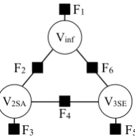
Fig. 1 displays an undirected factor graph, in which each factor is connected to the variables that it depends on. F1, F3, F5in this example are unary factors because each one scores the value of a single variable, while F2, F4, F6 are binary factors.
F2 F6
F5
F3
F1
F4
Vinf
[image:2.595.365.464.67.169.2]V2SA V3SE
Figure 1: Example of a factor graph. Black boxes represent factors, circles represent variables (infinitive, 2nd past, and 3rd present-tense forms of the same verb; different samples from the MRF correspond to different verbs). Binary factors evaluate how well one string can be transduced into another, summing over all transducer paths (i.e., alignments, which are not observed in training).
In our setting, we will assume that each unary factor is specified by aweighted finite-state au-tomaton(WFSA) whose weights fall in the semir-ing(R≥0,+,×). Thus the scoreF3(. . . , V2SA =
x, . . .)is the total weight of all paths in the F3’s WFSA that accept the string x ∈ Σ∗
2SA. Each path’s weight is the product of its component arcs’ weights, which are non-negative.
Similarly, we assume that each binary factor is specified by a weighted finite-state transducer (WFST). Such a model is essentially a generaliza-tion of stochastic edit distance (Ristad and Yian-ilos, 1996) in which the edit probabilities can be made sensitive to a finite summary of context.
Formally, a WFST is an automaton that resem-bles a weighted FSA, but it nondeterministically readstwostringsx, yin parallel from left to right. The score of(x, y)is given by the total weight of all accepting paths in the WFST that mapxtoy. For example, different paths may consider various monotonic alignments of x with y, and we sum over these mutually exclusive possibilities.1
A factor might depend onk >2variables. This requires a k-tape weighted finite-state machine (WFSM), an obvious generalization where each path readskstrings in some alignment.2
To ensure thatZis finite in equation (1), we can require each factor to be a“proper” WFSM, i.e., its accepting paths have finite total weight (even if the WFSM is cyclic, with infinitely many paths).
1Each string is said to be on a different “tape,” which has its own “read head,” allowing the WFSM to maintain a sep-arate position in each string. Thus, a path in a WFST may consume any number of characters fromxbefore consuming the next character fromy.
2Weighted acceptors and transducers are the casesk= 1 andk= 2, which are said to definerational languagesand
3.3 Parameters
Our probability model has trainable parameters: a vector offeature weightsθ∈R. Each arc in each WFSM has a real-valued weight that depends onθ. Thus, tuningθduring training will change the arc weights, hence the path weights, the factor func-tions, and the whole probability distributionp(A). Designing the probability model includes spec-ifying the topology and weights of each WFSM. Eisner (2002) explains how to specify and train such parameterized WFSMs. Typically, the weight of an arc is a simple sum likeθ12+θ55+
θ72, where θ12 is included on all arcs that share feature 12. However, more interesting parameter-izations arise if the WFSM is constructed by op-erations such as transducer composition, or from a weighted regular expression.
3.4 Power of the formalism
Factored finite-state string models (1) were orig-inally suggested by the second author, in Kempe et al. (2004). That paper showed that even in the unweighted case, such models could be used to en-code relations that could not be recognized by any
k-tape FSM. We offer a more linguistic example as a small puzzle. We invite the reader to spec-ify a factored model (consisting of three FSTs as in Fig. 1) that assigns positive probability to just those triples of character strings(x, y, z)that have the form (red ball, ball red, red), (white house,
house white, white), etc. This uses the auxiliary
variable Z to help encode a relation between X
andY that swaps words of unbounded length. By contrast, no FSM can accomplish such unbounded swapping, even with 3 or more tapes.
Such extra power might be linguistically useful. Troublingly, however, Kempe et al. (2004) also observed that the framework is powerful enough to express computationally undecidable problems.3
This implies that to work with arbitrary models, we will need approximate methods.4 Fortunately,
the graphical models community has already de-3Consider a simple model with two variables and two bi-nary factors:p(V1, V2)def= Z1 ·F1(V1, V2)·F2(V1, V2).
Sup-poseF1 is 1 or 0 according to whether its arguments are
equal. Under this model,p() < 1iff there exists a string
x 6= that can be transduced to itself by the unweighted transducerF2. This question can be used to encode any
in-stance of Post’s Correspondence Problem, so is undecidable. 4Notice that the simplest approximation to cure undecid-ability would be to impose an arbitrary maximum on string length, so that the random variables have a finite domain, just as in most discrete graphical models.
V
F U
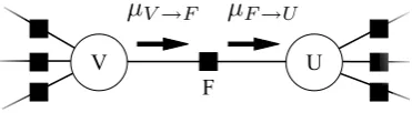
[image:3.595.324.510.65.116.2]µ
V→Fµ
F→UFigure 2: Illustration of messages being passed from variable to factor and factor to variable. Each message is represented by a finite-state acceptor.
veloped many such methods, to deal with the com-putational intractability (if not undecidability) of exact inference.
4 Approximate Inference
In this paper, we focus on howbelief propagation (BP)—a simple well-known method for approxi-mate inference in MRFs (Bishop, 2006)—can be used in our setting. BP in its general form has not yet been widely used in the NLP community.5
However, it is just a generalization to arbitrary
factor graphs of the familiar forward-backward al-gorithm (which operates only on chain-structured factor graphs). The algorithm becomes approxi-mate (and may not even converge) when the factor graphs have cycles. (In that case it is more prop-erly called “loopy belief propagation.”)
4.1 Belief propagation
We first sketch how BP works in general. Each variableV in the graphical model maintains a be-liefabout its value, in the form of a marginal dis-tribution p˜V over the possible values of V. The final beliefs are the output of the algorithm.
Beliefs arise from messages that are sent be-tween the variables and factors along the edges of the factor graph. VariableV sends factorF a mes-sageµV→F, which is an (unnormalized) probabil-ity distribution overV’s valuesv, computed by
µV→F(v) :=
Y
F0∈N(V),F06=F
µF0→V(v) (2)
whereN is the set of neighbors ofV in the graph-ical model. This message represents a consensus
ofV’s other neighboring factors concerningV’s
value. It is howV tellsFwhat its beliefp˜V would be ifF were absent. Informally, it communicates
toF:Here is what my value would be if it were up
to my other neighboring factorsF0to determine.
The factor F can then collect such incoming messages from neighboring variables and send its own message on to another neighborU. Such a messageµF→Usuggests good values forU, in the form of an (unnormalized) distribution over U’s valuesu, computed by
µF→U(u) := X
As.t.A[U]=u
F(A) Y
U0∈N(F),U06=U
µU0→F(A[U0])
(3) where A is an assignment to all variables, and
A[U] is the value of variable U in that assign-ment. This message representsF’s prediction of
U’s value based on itsotherneighboring variables
U0. Informally, via this message,F tellsU:Here
is what I would like your value to be, based on the messages that my other neighboring variables have sent me about their values, and how I would prefer you to relate to them.
Thus, each edge of the factor graph maintains two messages µV→F, µF→V. All messages are updated repeatedly, in some order, using the two equations above, until some stopping criterion is reached.6 Thebeliefsare then computed:
˜ pV(v)def=
Y
F∈N(V)
µF→V(v) (4)
If variable V is observed, then the right-hand sides of equations (2) and (4) are modified to tell
V that itmusthave the observed valuev. This is done by multiplying in an extra messageµobs→V that puts probability 1 on v7 and 0 on other
val-ues. That affectsothermessages and beliefs. The final belief at each variable estimates itsposterior
marginal under the MRF (1), given all
observa-tions.
4.2 Finite-state messages in BP
BothµV→F andµF→V are unnormalized distribu-tions over the possible values of V—in our case, strings. A distribution over strings is naturally represented by a WFSA. Thus, belief propagation translates to our setting as follows:
• Each message is a WFSA.
• Messages are typically initialized to a one-state WFSA that accepts all strings inΣ∗, each with 6Preferably when the beliefs converge to some fixed point (a local minimum of the Bethe free energy). However, con-vergence is not guaranteed.
7More generally, onallpossible observed variables.
weight 1.8
• Taking a pointwise product of messages toV in equation (2) corresponds to WFSA intersection.
• IfF in equation (3) is binary,9then there is only
oneU0. Then the outgoing message µF→U, a WFSA, is computed as domain(F◦µU0→F).
Here◦composes the factor WFST with the in-coming message WFSA, yielding a WFST that gives a joint distribution over (U, U0). The domain operator projects this WFST onto theU
side to obtain a WFSA, which corresponds to marginalizing to obtain a distribution overU.
• In general,F is a k-tape WFSM. Equation (3) “composes” k−1 of its tapes with k−1 in-coming messages µU0→F, to construct a joint
distribution over thekvariables inN(F), then projects onto thekthtape to marginalize over the
k−1U0variables and get a distribution overU. All this can be accomplished by the WFSM gen-eralized composition operator(Kempe et al., 2004).
After projecting, it is desirable to determinize the WFSA. Otherwise, the summation in (3) is only implicit—the summands remain as distinct paths in the WFSA10—and thus the WFSAs would
get larger and larger as BP proceeds. Unfortu-nately, determinizing a WFSA still does not guar-antee a small result. In fact it can lead to expo-nential blowup, or even infinite blowup.11 Thus,
in practice we recommend against determinizing the messages, which may be inherently complex. To shrink a message, it is safer toapproximateit with a small deterministic WFSA, as discussed in the next section.
4.3 Approximation of messages
In our domain, it is possible for the finite-state messages togrow unboundedly in sizeas they flow around a cycle. After all, our messages are not just multinomial distributions over a fixed finite 8This is an (improper) uniform distribution overΣ∗.
Al-though isnota proper WFSA (see section 3.2), there is an upper bound on the weights it assigns to strings. That guar-antees that all the messages and beliefs computed by (2)–(4) will be proper FSMs, provided that all the factors are proper WFSMs.
9If it is unary, (3) trivially reduces toµ
F→U=F. 10The usual implementation of projection does not change the topology of the WFST, but only deletes theU0part of its
arc labels. Thus, multiple paths that accept the same value of
U remain distinct according to the distinct values ofU0that
they were paired with before projection.
set. They are distributions over the infinite setΣ∗. A WFSA represents this in finite space, but more complex distributions require bigger WFSAs, with more distinct states and arc weights.
Facing the same problem for distributions over the infinite setR, Sudderth et al. (2002) simplified each message µV→F, approximating a complex Gaussian mixture by using fewer components.
We could act similarly, variationally approxi-mating a large WFSA P with a smaller one Q. Choose a family of message approximations (such as bigram models) by specifying the topology for a (small) deterministic WFSA Q. Then choose
Q’s edge weights to minimize the KL divergence KL(PkQ). This can be done in closed form.12
Another possible procedure—used in the ex-periments of this paper—approximatesµV→F by pruning it back to a finite set of most plausible strings.13 Equation (2) requests an intersection
of several WFSAs, e.g.,µF1→V ∩µF2→V ∩ · · ·.
List all strings that appear on any of the 1000-best paths in any of these WFSAs, removing du-plicates. LetQ¯be a uniform distribution over this combined list of plausible strings, represented as a determinized, minimized, acyclic WFSA. Now approximate the intersection of equation (2) as
(( ¯Q∩µF1→V)∩µF2→V)∩ · · ·. This is efficient
to compute and has the same topology asQ¯.
5 Training the Model Parameters
Any standard training method for MRFs will transfer naturally to our setting. In all cases we draw on Eisner (2002), who showed how to train the parametersθof asingleWFST,F, to (locally) maximize the joint or conditional probability of fully or partially observed training data. This in-volves computing the gradient of that likelihood function with respect toθ.14
12See Li et al. (2009, footnote 9) for a sketch of the con-struction, which finds locally normalized edge weights. Or ifQis large but parameterized by some compact parameter vectorφ, so we are only allowed to control its edge weights viaφ, then Li and Eisner (2009, section 6) explain how to minimize KL(PkQ)by gradient descent. In both casesQ
must be deterministic.
We remark that if a factor F were specified by a syn-chronous grammar rather than a WFSM, then its outgoing messages would be weighted context-free languages. Exact intersection of these is undecidable, but they too can be ap-proximated variationally by WFSAs, with the same methods. 13We are also considering other ways of adaptively choos-ing the topology of WFSA approximations at runtime, partic-ularly in conjunction with expectation propagation.
14The likelihood is usually non-convex; even when the two strings are observed (supervised training), their accepting
We must generalize this to train a product of WFSMs. Typically, training data for an MRF (1) consists of some fully or partially observed IID samples of the joint distributionp(V1, . . . Vn). It is well-known how to tune an MRF’s parametersθ
by stochastic gradient descent to locally maximize the probability of this training set, even though both the probability and its gradient are in general intractable to compute in an MRF. The gradient is a sum of quantities, one for each factorFj. While the summand forFj cannot be computed exactly, it can be estimated using the BP messages toFj. Roughly speaking, the gradient forFjis computed much as in supervised training (see above), but treating any messageµVi→Fj as an uncertain ob-servation ofVi—a form of noisy supervision.15
Our concerns about training are the same as for any MRF. First of all, BP is approximate. Kulesza and Pereira (2008) warn that its estimates of the gradient can be misleading. Second, semi-supervised training (which we will attempt below) is always difficult and prone to local optima. As in EM, a small number of supervised examples for some variable may be drowned out by many nois-ily reconstructed examples.
Faster and potentially more stable approaches include the piecewise training methods of Sut-ton and McCallum (2008), which train the factors independently or in small groups. In the semi-supervised case, each factor can be trained on only the supervised forms available for it. It might be useful to reweight the trained factors (cf. Smith et al. (2005)), or train the factors consecutively (cf. Fahlman and Lebiere (1990)), in a way that mini-mizes the loss of BP decoding on held-out data.
6 Comparison With Other Approaches 6.1 Multi-tape WFSMs
In principle, one could use a 100-tape WFSM to jointly model the 100 distinct forms of a typical Polish verb. In other words, the WFSM would de-scribe the distribution of a random variable ~V =
hV1, . . . , V100i, where each Vi is a string. One would train the parameters of the WFSM on a sample of~V, each sample being a fully or partially observed paradigm for some Polish verb. The re-sulting distribution could be used to infer missing forms for these or other verbs.
As a simple example, either a morphological generator or a morphological analyzer might need the probability thatkrzyczałobyis the neuter third-person singular conditional imperfective of
krzy-cze´c, despite never having observed it in training.
The model determines this probability based on other observed and hypothesized forms of
krzy-cze´c, using its knowledge of how neuter
third-person singular conditional imperfectives are re-lated to these other forms in other verbs.
Unfortunately, such a 100-tape WFSM would be huge, with an astronomical number of arcs (each representing a possible 100-way edit opera-tion). Our approach is to factor the problem into a number of (e.g.) pairwise relationships among the verb forms. Using a factored distribution has sev-eral benefits over thek-tape WFSM: (1) a smaller representation in memory, (2) a small number of parameters to learn, (3) efficient approximate computation that takes advantage of the factored structure, (4) the ability to reuse WFSAs and WF-STs previously developed for smaller problems, (5) additional modeling power.
6.2 Simpler graphical models on strings Some previous researchers have used factored joint models of several strings. To our knowledge, they have all chosen acyclic, directed graphical models. The acyclicity meant that exact inference was at least possible for them, if not necessarily ef-ficient. The factors in these past models have been WFSTs (though typically simpler than the ones we will use).
Many papers have used cascades of probabilis-tic finite-state transducers. Such a cascade may be regarded as a directed graphical model with a linear-chain structure. Pereira and Riley (1997) built a speech recognizer in this way, relating acoustic to phonetic to lexical strings. Simi-larly, Knight and Graehl (1997) presented a gen-erative cascade using 4 variables and 5 factors:
p(w, e, j, k, o)=defp(w)·p(e|w)·p(j|e)·p(k|j)
·p(o|k)whereeis an English word sequence,w
its pronunciation,ja Japanese version of the pro-nunciation,ka katakana rendering of the Japanese pronunciation, andoan OCR-corrupted version of the katakana. Knight and Graehl used finite-state operations to perform inference at test time, ob-servingoand recovering the most likelyw, while marginalizing oute,j, andk.
Bouchard-Cˆot´e et al. (2009) reconstructed
an-cient word forms given modern equivalents. They used a directed graphical model, whose tree struc-ture reflected the evolutionary development of the modern languages, and which included latent vari-ables for historical intermediate forms that were never observed in training data. They used Gibbs sampling rather than an exact solution (possible on trees) or a variational approximation (like our BP). Our work seeks to be general in terms of the graphical model structures used, as well as effi-cient through the use of BP with approximate mes-sages. We also seek to avoid local normalization, using a globally normalized model.16
6.3 Unbounded objects in graphical models We distinguish our work from “dynamic” graph-ical models such as Dynamic Bayesian Networks and Conditional Random Fields, where the string
brechenwould be represented by creating 7
letter-valued variables. Those methods can represent strings (or paths) of any length—but the length for each training or test string must be specified in ad-vance, not inferred. Furthermore, it is awkward and costly to model unknown alignments, since the variables are position-specific, and any posi-tion inbrechen could in principle align with any position inbrichst. WFSTs are a much more natu-ral and flexible model of string pairs.
We also distinguish our work from current non-parametric Bayesian models, which sometimes generate unbounded strings, trees, or grammars. If they generate two unbounded objects, they model their relationship by a single synchronous genera-tion process (akin to Secgenera-tion 6.1), rather than by a globally normalized product of overlapping fac-tors.
7 Experiments
To study our approach, we conducted initial ex-periments that reconstruct missing word forms in morphological paradigms. In inflectional
mor-phology, each uninflected verb form (lemma) is
associated with a vector of forms that are inflected for tense, person, number, etc. Some inflected forms may be observed frequently in natural text, others rarely. Two variables that are usually pre-dictable from each other may or may not keep this relationship in the case of an irregular verb.
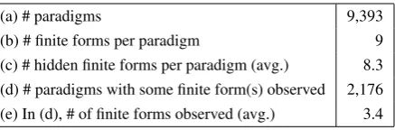
(a) # paradigms 9,393
(b) # finite forms per paradigm 9
[image:7.595.78.297.61.133.2](c) # hidden finite forms per paradigm (avg.) 8.3 (d) # paradigms with some finite form(s) observed 2,176 (e) In (d), # of finite forms observed (avg.) 3.4
Table 1: Statistics of our training data.
Our task is to reconstruct (generate) specific un-observed morphological forms in a paradigm by learning from observed ones. This is a particu-larly interesting semisupervised scenario, because different subsets of the variables are observed on different examples.
7.1 Experimental data
We used orthographic rather than phonological forms. We extracted morphological paradigms for all 9393 German verbs in the CELEX morpholog-ical database. Each paradigm lists 5 present-tense and 4 past-tense indicative forms, as well as the verb’s lemma, for a total of 10 string-valued vari-ables.17 In each paradigm, we removed, or hid,
verb forms that occur only rarely in natural text, i.e, verb forms with a small frequency figure pro-vided by CELEX.18All paradigms other thansein
(’to be’) were now incompletely observed. Table 1 gives some statistics.
7.2 Model factors and parameters
Our current MRF uses only binary factors. Each factor is a WFST that is trained to relate 2 of the 10 variables (morphological forms). Each WFST can score an aligned pair using a log-linear model that counts features in a sliding 3-character window. To score an unaligned pair, it sums over all pos-sible alignments. Specifically, our WFST topol-ogy and parameterization follow the state-of-the-art approach tosupervisedmorphology in Dreyer et al. (2008), although we dropped some of their features to speed up these early experiments.19 We
17Some pairs of forms are always identical in German, hence are treated as a single form by CELEX. We likewise use a single variable—these are the “1,3” variables in Fig. 3. Occasionally a form is listed as UNKNOWN. We neither train nor evaluate on such forms, although the model will still predict them.
18The frequency figure for each word form is based on counts in the Mannheim News corpus. We hide forms with frequency<10.
19We dropped their latent classes and regions as well as features that detected which characters were orthographic vowels. Also, we retained their “target language model fea-tures” only in the baseline “U” model, since elsewhere they
implemented and manipulated all WFSMs using the OpenFST library (Allauzen et al., 2007).
7.3 Training in the experiments
We trained θ on the incompletely observed paradigms. As suggested in section 5, we used a variant of piecewise pseudolikelihood training (Sutton and McCallum, 2008). Suppose there is a binary factorF attached to formsU andV. For any value ofθ, we can define pUV(U | V) from the tiny MRF consisting only of U, V, and F. We can therefore compute the goodness LUV def=
logpUV(ui|vi)+logV U(vi|ui),20summed over
allobserved(U, V)pairs in training data. We
at-tempted to tuneθto maximize the totalLUV over allU, V pairs,21 regularized by subtracting||θ||2. Note that different factors thus enjoyed different amounts of observed training data, but training was fully supervised (except for the unobserved alignments betweenuiandvi).
7.4 Inference in the experiments
At test time, we are given each lemma (e.g.
brechen) and all its observed (frequent) inflected
forms (e.g.,brachen,bricht,. . . ), and are asked to predict the remaining (rarer) forms (e.g., breche,
brichst, . . .).
We run approximate joint inference using be-lief propagation.22 We extract our output from the
final beliefs: for each unseen variableV, we pre-seemed to hurt in our current training setup.
We followed Dreyer et al. (2008) in slightly pruning the space of possible alignments. We compensated by replacing their WFST,F, with the unionF∪10−12(0.999Σ×Σ)∗.
This ensured that the factor could still map any string to any other string (though perhaps with very low weight), guaran-teeing that the intersection at the end of section 4.3 would be non-empty.
20The second term is omitted ifV is the lemma. We do not train the model to predict the lemma since it is always observed in test data.
21Unfortunately, just before press time we discovered that this was not quite what we had done. A shortcut in our im-plementation trainedpUV(U | V)andpV U(V | U) sepa-rately. This let them make different use of the (unobserved) alignments—so that even if each individually liked the pair
(u, v), they might not have been able to agree on the same accepting path for it at test time. This could have slightly harmed our joint inference results, though not our baselines.
dict its value to beargmaxvp˜V(v). This predic-tion considers the values of all other unseen vari-ables but sums over their possibilities. This is the Bayes-optimal decoder for our scoring function, since that function reports the fraction of
individ-ual formsthat were predictedperfectly.23
7.5 Model selection of MRF topology
It is hard to knowa prioriwhat the causal relation-ships might be in a morphological paradigm. In principle, one would like toautomaticallychoose which factors to have in the MRF. Or one could start with many factors, but use methods such as those suggested in section 5 to learn that certain less useful factors should be left weak to avoid confusing loopy BP.
For our present experiments, we simply com-pared several fixed model topologies (Fig. 3). These were variously unconnected (U), chain graphs (C1,. . . , C4), trees (T1, T2), or loopy graphs (L1,. . . , L4). We used several factor graphs that differ only by one or two added factors and compared the results. The graphs were designed by hand; they connect some forms with similar morphological properties more or less densely.
We trained different models using the observed forms in the 9393 paradigms as training data. The first 100 paradigms were then used as develop-ment data for model selection:24 we were given
the answers to their hidden forms, enabling us to compare the models. The best model was then evaluated on the 9293 remaining paradigms. 7.6 Development data results
The models are compared on development data in Table 2. Among the factor graphs we evalu-ated, we find that L4 (see Fig. 3) performs best overall (whole-word accuracy 82.1). Note that the unconnected graph U does not perform very well (69.0), but using factor graphs with more connect-ing factors generally helps overall accuracy (see C1–C3). Note, however, that in some cases the ad-ditional structure hurts: The chain model C4 and the loopy model L1 perform relatively badly. The 23If we instead wished to maximize the fraction of entire paradigms that were predicted perfectly, then we would have approximated full MAP decoding over the paradigm (Viterbi decoding) by using max-product BP. Other loss functions (e.g., edit distance) would motivate other decoding methods. 24Using these paradigms was simply a quick way to avoid model selection by cross-validation. If data were really as sparse as our training setup pretends (see Table 2), then 100 complete paradigms would be too valuable to squander as mere development data.
(U) 1 Pres Past Singular Plural 2 3 1,3 2 1,3 2 2 1,3 1 2 3 1,3 2 1,3 2 2 1,3 1 2 3 1,3 2 1,3 2 2 1,3
(C1) (C2) (C3)
1 2 3 1,3 2 1,3 2 2 1,3 1 2 3 1,3 2 1,3 2 2 1,3 (C4) 1 2 3 1,3 2 1,3 2 2 1,3 (T1) 1 2 3 1,3 2 1,3 2 2 1,3 (T2) (L1) 1 2 3 1,3 2 1,3 2 2 1,3 (L2) 1 2 3 1,3 2 1,3 2 2 1,3 1 2 3 1,3 2 1,3 2 2 1,3 (L3) Pres Past Pres Past Pres Past Pres Past
[image:8.595.311.526.68.225.2]Singular Plural 1 2 3 1,3 2 1,3 2 2 1,3 (L4)
Figure 3: The graphs that we evaluate on development data. The nodes represent morphological forms, e.g. the first node in the left of each graph represents the first person singular present. Each variable is also connected to the lemma (not shown). See results in Table 2.
reason for such a performance degradation is that undertrained factors were used: The factors relat-ing second-person to second-person forms, for ex-ample, are trained from only 8 available examples. Non-loopy models always converge (exactly) in one iteration (see footnote 22). But even our loopy models appeared to converge in accuracy within two iterations. Only L3 and L4 required the sec-ond iteration, which made tiny improvements.
7.7 Test data results
Based on the development results, we selected model L4 and tested on the remaining 9293 paradigms.
We regard the unconnected model U as a base-line to improve upon. We also tried a rather differ-ent baseline as in (Dreyer et al., 2008). We trained the machine translation toolkit Moses (Koehn et al., 2007) to translate groups of letters rather than groups of words (“phrases”). For each form f
to be predicted, we trained a Moses model on all supervised form pairs (l, f) available in the data, to learn a prediction for the form given the lemmal. The M,3 condition restricted Moses use “phrases” no longer than 3 letters, comparable to our own trigram-based factors (see section 7.2). M,15 could use up to 15 letters.
bet-Unconn. Chains Trees Loops
U C1 C2 C3 C4 T1 T2 L1 L2 L3 L4
69.0 72.9 73.4 74.8 65.2 78.1 78.7 62.3 79.6 78.9 82.1
Table 2: Whole-word accuracies of the different models in reconstructing the missing forms in morphological paradigms, here on 100 verbs (development data). The names refer to the graphs in Fig. 3. We selected L4 as final model (Table 3).
Form # obs. M,3 M,15 U L4
2.Sg.Pa. 4 0.0 0.2 0.8 69.7
2.Pl.Pa. 9 0.9 1.1 1.4 45.6
2.Sg.Pr. 166 49.4 62.6 74.7 90.5
1.Sg.Pr. 285 99.6 98.8 99.3 97.2
1,3.Pl.Pa. 673 46.5 78.3 75.0 75.6
1,3.Sg.Pa. 1124 65.0 88.8 84.0 74.8
2.Pl.Pr. 1274 98.3 99.2 99.0 96.4
3.Sg.Pr. 1410 91.0 95.9 95.2 88.2
1,3.Pl.Pr. 1688 99.8 98.9 99.8 98.0
[image:9.595.117.484.62.109.2]All 6633 59.2 67.3 68.0 81.2 Table 3: Whole-word accuracies on the missing forms from 9293 test paradigms. The Moses baselines and our un-connected model (U) predict each form separately from the lemma, which is always observed. L4 uses all observations jointly, running belief propagation for decoding. Moses,15 memorizes phrases of length up to 15, all other models use max length 3. The table is sorted by the column “# obs.”, which reports the numbers of observations for a given form. ter by exploiting other observed or latent forms. By contrast, well-trained forms were already easy enough for the M and U models that L4 had little new to offer and in fact suffered from its approxi-mate training and/or inference.
Leaving aside the comparisons, it was useful to confirm that loopy BP could be used in this set-ting at all. 8014 of the 9293 test paradigms had
≤ 2 observed forms (in addition to the lemma) but≥7missing forms. One might have expected that loopy BP would have failed to converge, or converged to the wrong thing. Nonetheless, it achieved quite respectable success at exactly pre-dicting various inflected forms.
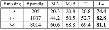
For the curious, Table 4 shows accuracies grouped by different categories of paradigms, where the category is determined by the number of missing forms to predict. Most paradigms fall in the category where 7 to 9 forms are missing, so the accuracies in that line are similar to the overall accuracies in Table 3.
8 Conclusions
We have proposed that one can jointly model sev-eral multiple strings by using Markov Random Fields. We described this formally as an
undi-# missing # paradig. M,3 M,15 U L4
1–3 205 20.3 20.8 26.8 74.4 4–6 1037 44.2 50.5 52.7 82.8 7–9 8014 60.6 68.8 69.4 81.1
Table 4: Accuracy on test data, reported separately for paradigms in which 1–3, 4–6, or 7–9 forms are missing. Missing words have CELEX frequency count<10; these are the ones to predict. (The numbers in col. 2 add up to 9256, not 9293, since some paradigms are incomplete in CELEX to begin with, with no forms to be removed or evaluated.)
rected graphical model with string-valued vari-ables and whose factors (potential functions) are defined by weighted finite-state transducers. Each factor evaluates some subset of the strings.
Approximate inference can be done by loopy belief propagation. The messages take the form of weighted finite-state acceptors, and are con-structed by standard operations. We explained why the messages might become large, and gave methods for approximating them with smaller messages. We also discussed training methods.
We presented some pilot experiments on the task of jointly predicting multiple missing verb forms in morphological paradigms. The factors were simplified versions of statistical finite-state models for supervised morphology. Our MRF for this task might be used not only to conjugate verbs (e.g., in MT), but to guide further learning of morphology—either active learning from a hu-man or semi-supervised learning from the distri-butional properties of a raw text corpus.
Our modeling approach is potentially applicable to a wide range of other tasks, including translit-eration, phonology, cognate modeling, multiple-sequence alignment and system combination.
[image:9.595.306.526.156.218.2]References
Cyril Allauzen, Michael Riley, Johan Schalkwyk, Wo-jciech Skut, and Mehryar Mohri. 2007. OpenFst: A general and efficient weighted finite-state transducer library. InProc. of CIAA, volume 4783 ofLecture Notes in Computer Science, pages 11–23.
Christopher M. Bishop. 2006. Pattern Recognition and Machine Learning. Springer.
Alexandre Bouchard-Cˆot´e, Thomas L. Griffiths, and Dan Klein. 2009. Improved reconstruction of pro-tolanguage word forms. In Proc. of HLT-NAACL, pages 65–73, Boulder, Colorado, June. Association for Computational Linguistics.
Fabien Cromier`es and Sadao Kurohashi. 2009. An alignment algorithm using belief propagation and a structure-based distortion model. InProc. of EACL, pages 166–174, Athens, Greece, March. Association for Computational Linguistics.
Markus Dreyer, Jason Smith, and Jason Eisner. 2008. Latent-variable modeling of string transductions with finite-state methods. InProc. of EMNLP, Hon-olulu, Hawaii, October.
Jason Eisner. 2002. Parameter estimation for prob-abilistic finite-state transducers. In Proc. of ACL, pages 1–8, Philadelphia, July.
Scott E. Fahlman and Christian Lebiere. 1990. The cascade-correlation learning architecture. Technical Report CMU-CS-90-100, School of Computer Sci-ence, Carnegie Mellon University.
Andr´e Kempe, Jean-Marc Champarnaud, and Jason Eisner. 2004. A note on join and auto-intersection of n-ary rational relations. In Loek Cleophas and Bruce Watson, editors, Proceedings of the Eind-hoven FASTAR Days (Computer Science Techni-cal Report 04-40). Department of Mathematics and Computer Science, Technische Universiteit Eind-hoven, Netherlands.
Kevin Knight and Jonathan Graehl. 1997. Machine transliteration. InProc. of ACL, pages 128–135. Philipp Koehn, Hieu Hoang, Alexandra Birch, Chris
Callison-Burch, Marcello Federico, Nicola Bertoldi, Brooke Cowan, Wade Shen, Christine Moran, Richard Zens, Chris Dyer, Ondrej Bojar, Alexandra Constantin, and Evan Herbst. 2007. Moses: Open source toolkit for statistical machine translation. In Proc. of ACL, Companion Volume, pages 177–180, Prague, Czech Republic, June. Association for Com-putational Linguistics.
Alex Kulesza and Fernando Pereira. 2008. Structured learning with approximate inference. In Proc. of NIPS.
Zhifei Li and Jason Eisner. 2009. First- and second-order expectation semirings with applications to minimum-risk training on translation forests. In Proc. of EMNLP.
Zhifei Li, Jason Eisner, and Sanjeev Khudanpur. 2009. Variational decoding for statistical machine transla-tion. InProc. of ACL.
Mehryar Mohri. 1997. Finite-state transducers in lan-guage and speech processing. Computational Lin-guistics, 23(2).
Fernando C. N. Pereira and Michael Riley. 1997. Speech recognition by composition of weighted fi-nite automata. In Emmanuel Roche and Yves Schabes, editors,Finite-State Language Processing. MIT Press, Cambridge, MA.
Eric Sven Ristad and Peter N. Yianilos. 1996. Learn-ing strLearn-ing edit distance. Technical Report CS-TR-532-96, Princeton University, Department of Com-puter Science, October.
David Smith and Jason Eisner. 2008. Dependency parsing by belief propagation. InProc. of EMNLP. Andrew Smith, Trevor Cohn, and Miles Osborne.
2005. Logarithmic opinion pools for conditional random fields. InProc. of ACL, pages 18–25, June. Erik B. Sudderth, Alexander T. Ihler, Er T. Ihler,
William T. Freeman, and Alan S. Willsky. 2002. Nonparametric belief propagation. In Proc. of CVPR, pages 605–612.
Charles Sutton and Andrew McCallum. 2004. Collec-tive segmentation and labeling of distant entities in information extraction. InICML Workshop on Sta-tistical Relational Learning and Its Connections to Other Fields.
Charles Sutton and Andrew McCallum. 2008. Piece-wise training for structured prediction. Machine Learning. In submission.