Proceedings of the 2019 Conference on Empirical Methods in Natural Language Processing 4069
Don’t Take the Easy Way Out:
Ensemble Based Methods for Avoiding Known Dataset Biases
Christopher Clark∗, Mark Yatskar†, Luke Zettlemoyer∗
∗Paul G. Allen School of CSE, University of Washington
{csquared, lsz}@cs.uw.edu
†Allen Institute for Artificial Intelligence, Seattle WA
Abstract
State-of-the-art models often make use of su-perficial patterns in the data that do not gener-alize well to out-of-domain or adversarial set-tings. For example, textual entailment mod-els often learn that particular key words im-ply entailment, irrespective of context, and vi-sual question answering models learn to pre-dict prototypical answers, without considering evidence in the image. In this paper, we show that if we have prior knowledge of such biases, we can train a model to be more robust to do-main shift. Our method has two stages: we (1) train a naive model that makes predictions ex-clusively based on dataset biases, and (2) train a robust model as part of an ensemble with the naive one in order to encourage it to focus on other patterns in the data that are more likely to generalize. Experiments on five datasets with out-of-domain test sets show significantly im-proved robustness in all settings, including a 12 point gain on a changing priors visual ques-tion answering dataset and a 9 point gain on an adversarial question answering test set.
1 Introduction
While recent neural models have shown remark-able results, these achievements have been tem-pered by the observation that they are often ex-ploiting dataset-specific patterns that do not gen-eralize well to out-of-domain or adversarial set-tings. For example, entailment models trained on MNLI (Bowman et al., 2015) will guess an an-swer based solely on the presence of particular keywords (Gururangan et al., 2018) or whether sentences pairs contain the same words (
Mc-Coy et al., 2019), while QA models trained on
SQuAD (Rajpurkar et al.,2016) tend to select text near question-words as answers, regardless of con-text (Jia and Liang,2017).
We refer to these kinds of superficial patterns as bias. Models that rely on bias can perform
well on in-domain data, but are brittle and easy to fool (e.g., SQuAD models are easily distracted by irrelevant sentences that contain many question words). Recent concern about dataset bias has led researchers to re-examine many popular datasets, resulting in the discovery of a wide variety of bi-ases (Agrawal et al.,2018;Anand et al.,2018;Min et al.,2019;Schwartz et al.,2017).
In this paper, we build on these works by show-ing that, once a dataset bias has been identified, we can improve the out-of-domain performance of models by preventing them from making use of that bias. To do this, we use the fact that these bi-ases can often be explicitly modelled with simple, constrained baseline methods to factor them out of a final model through ensemble-based training.
What color is the grass?
Bias-Only Model Robust Model
Ensemble
Data Gradients
Brown Yellow Gold Green Blue Gray Other
p(answer|model)
Brown Yellow Gold Green Blue Gray Other
p(answer|ensemble)
Brown Yellow Gold Green Blue Gray Other
p(answer|bias)
Training Loss
Training
Prediction
[image:2.595.89.509.64.277.2]Evaluation
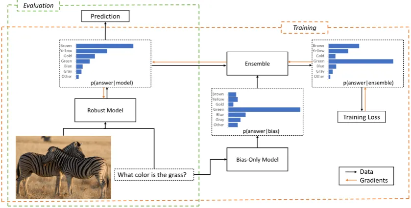
Figure 1: An example of applying our method to a Visual Question Answering (VQA) task. We assume predicting green for the given question is almost always correct on the training data. To prevent a model from learning this bias, we first train a bias-only model that only uses the question as input, and then train a robust model in an ensemble with the bias-only model. Since the bias-only model will have already captured the target pattern, the robust model has no incentive to learn it, and thus does better on test data where the pattern is not reliable.
2019;Jia and Liang,2017), which were designed to break models that adopt superficial strategies on well known textual entailment (Bowman et al.,
2015), reading comprehension (Rajpurkar et al.,
2016), and VQA (Antol et al.,2015) datasets. We additionally construct a new QA challenge dataset, TriviaQA-CP (for TriviaQA changing pri-ors). This dataset was built by holding out ques-tions from TriviaQA (Joshi et al.,2017) that ask about particular kinds of entities from the train set, and evaluating on those questions in the dev set, in order to challenge models to generalize between different types of questions.
We are able to improve out-of-domain perfor-mance in all settings, including a 6 and 9 point gain on the two QA datasets. On the VQA chal-lenge set, we achieve a 12 point gain, compared to a 3 point gain from prior work. In general, we find using an ensembling method that can dynam-ically choose when to trust the bias-only model is the most effective, and we present synthetic exper-iments and qualitative analysis to illustrate the ad-vantages of that approach. We release our datasets and code to facilitate future work.1
2 Related Work
Researchers have raised concerns about bias in many datasets. For example, many joint
natu-1github.com/chrisc36/debias
ral language processing and vision datasets can be partially solved by models that ignore the vi-sion aspect of the task (Jabri et al., 2016; Zhang et al., 2016;Anand et al., 2018;Caglayan et al.,
2019). Some questions in recent multi-hop QA datasets (Yang et al.,2018;Welbl et al.,2018) can be solved by single-hop models (Chen and Dur-rett,2019;Min et al.,2019). Additional examples include story completion (Schwartz et al., 2017) and multiple choice questions (Clark et al.,2016,
2018). Recognizing that bias is a concern in di-verse domains, our work is the first to perform an evaluation across multiple datasets spanning lan-guage and vision.
Recent dataset construction protocols have tried to avoid certain kinds of bias. For example, both CoQA (Reddy et al.,2019) and QuAC (Choi et al.,
2018) take steps to prevent annotators from us-ing words that occur in the context passage, VQA 2.0 (Goyal et al., 2018) selects examples to limit the effectiveness of question-only models, and others have filtered examples solvable by simple baselines (Yang et al.,2018;Zhang et al.,2018b;
Recent work has focused on biases that come from ignoring parts of the input (e.g., guessing the answer to a question before seeing the evi-dence). Solutions include generative objectives to force models to understand all the input (Lewis
and Fan, 2019), carefully designed model
archi-tecture (Agrawal et al.,2018;Zhang et al.,2016), or adversarial removal of class-indicative features from model’s internal representations ( Ramakrish-nan et al., 2018; Zhang et al., 2018a; Belinkov
et al., 2019; Grand and Belinkov, 2019). In
contrast, we consider biases beyond partial-input cases (Feng et al., 2019), and show our method is superior on VQA-CP. Concurrently, He et al.
(2019) also suggested using a product-of-experts ensemble to train unbiased models, but we con-sider a wider variety of ensembling approaches and test on additional domains.
A related task is preventing models from us-ing particular problematic dataset features, which is often studied from the perspective of fair-ness (Zhao et al., 2017; Burns et al., 2018). A popular approach is to use an adversary to remove information about a target feature, often gender or ethnicity, from a model’s internal representa-tions (Edwards and Storkey, 2016; Wang et al.,
2018;Kim et al.,2019). In contrast, the biases we consider are related to features that are essential to the overall task, so they cannot simply be ignored. Evaluating models on out-of-domain examples built by applying minor perturbations to exist-ing examples has also been the subject of recent study (Szegedy et al., 2014; Belinkov and Bisk,
2018;Carlini and Wagner, 2018;Glockner et al.,
2018). The domain shifts we consider involve larger changes to the input distribution, built to un-cover higher-level flaws in existing models.
3 Methods
This section describes the two stages of our method, (1) building a bias-only model and (2) us-ing it to train a robust model through ensemblus-ing.
3.1 Training a Bias-Only Model
The goal of the first stage is to build a model that performs well on training data, but is likely to per-form very poorly on the out-of-domain test set. Since we assume we do not have access to ex-amples from the test set, we must apply a-priori knowledge to meet this goal.
The most straightforward approach is to
iden-tify a set of features that are correlated with the class label during training, but are known to be un-correlated or antiun-correlated with the label on the test set, and then train a classifier on those fea-tures.2For example, our VQA-CP (Agrawal et al.,
2018) bias-only model (see Section5.2) uses the question type as input, because the correlations be-tween question types and answers is very different in the train set than the test set (e.g., 2 is a common answer to “How many...” questions on the train set, but is rare for such questions on the test set).
However, a benefit of our method is that the bias can be modelled using any kind of predictor, giv-ing us a way to capture more complex intuitions. For example, on SQuAD our bias-only model op-erates on a view of the input built from TF-IDF scores (see Section5.4), and on our changing prior TriviaQA dataset our bias-only model makes use of a pre-trained named entity recognition (NER) tagger (see Section5.5).
3.2 Training a Robust Model
This stage trains a robust model that avoids using the method learned by the bias-only model.
3.2.1 Problem Definition
We assumentraining exampleshx1, x2, . . . , xni,
each of which has an integer labelyi, whereyi ∈ {1,2, . . . , C}andC is the number of classes. We additionally assume a trained bias-only pre-dictor, h, where h(xi) = bi = hbi1, bi2, ..biCi
andbij is the bias-only model’s predicted
proba-bility of classj for examplei. Finally we have a second predictor function, f, with parameters θ, wheref(xi, θ) =piandpiis a similar probability
distribution over the classes. Our goal is to con-struct a training objective to optimizeθso that f
will learn to select the correct class without using the strategy captured by the bias-only model.
3.2.2 General Approach
We train an ensemble of h and f. In particular, for each example, a new class distribution, pˆi, is
computed by combiningpi andbi. During
train-ing, the loss is computed using pˆi and the
gradi-ents are backproped throughf. During evaluation
f is used alone. We propose several different en-sembling methods.
2Since the bias-only model is trained on the same
3.2.3 Bias Product
Our simplest ensemble is a product of ex-perts (Hinton,2002):
ˆ
pi =softmax(log(pi) + log(bi))
Equivalently,pˆi ∝pi◦bi, where◦is
element-wise multiplication.
Probabilistic Justification: For a given ex-ample,x, letxb be the bias of the example. That is, it is the features we will use in our bias-only model. Let x−b be a view of the example that captures all information about that example except the bias. Assume that x−b and xb are conditionally independent given the label,c. Then to computep(c|x)we have:
p(c|x) = p(c|xb, x−b) (1)
∝ p(c|x−b)p(xb|c, x−b) (2)
= p(c|x−b)p(xb|c) (3)
= p(c|x−b)p(c|x
b)p(xb)
p(c) (4)
∝ p(c|x−b)p(c|x
b)
p(c) (5)
Where 2 is from applying Bayes Rule while conditioning on x−b, 3 follows from the condi-tional independence assumption, and 4 applies Bayes Rule a second time top(xb|c).
We cannot directly model p(c|x−b) because it is usually not possible to create a view of the data that excludes the bias. Instead, with the goal of encouraging the model to fall into the role of com-putingp(c|x−b), we compute p(c|xb)/p(c) using the bias-only model, and train the product of the two models to computep(c|x).
In practice, we ignore the p(c) factor because, on our datasets, either the classes are uniformly distributed (MNLI), the bias-only model cannot easily capture a class prior since it is using a pointer network (QA), or because we want to re-move class priors from model anyway (VQA).
3.2.4 Learned-Mixin
The assumption of conditional independence (Equation 3) will often be too strong. For exam-ple, in some cases the robust model might be able to predict the bias-only model will be unreliable for certain kinds of training examples. We find that this can cause the robust model to selectively adjust its behavior in order to compensate for the
inaccuracy of the bias-only model, leading to er-rors in the out-of-domain setting (see Section5.1). Instead we allow the model to explicitly deter-mine how much to trust the bias given the input:
ˆ
pi=softmax(log(pi) +g(xi) log(bi))
whereg is a learned function. We compute g as
softplus(w·hi)wherewis a learned vector,hiis
the last hidden layer of the model for examplexi,
and thesoftplus(x) = log(1+ex)function is used to prevent the model reversing the bias by multi-plying it by a negative weight. wis trained with the rest of the model parameters. This reduces to bias product wheng(xi) = 1.
A difficulty with this method is that the model could learn to integrate the bias into pi and set g(xi) = 0. We find this does sometimes occurs in
practice, and our next method alleviates this chal-lenge.
3.2.5 Learned-Mixin +H
To prevent the learned-mixin ensemble from ig-noringbi, we add an entropy penalty to the loss:
R=wH(softmax(g(xi) log(bi)))
WhereH(z) = −P
jzjlog(zj)is the entropy
andwis a hyperparameter. Penalizing the entropy encourages the bias component to be non-uniform, and thus have a greater impact on the ensemble.
4 Evaluation Methodology
We evaluate our methods on several datasets that have out-of-domain test sets. Some of these tasks, such as HANS (McCoy et al.,2019) or Adversar-ial SQuAD (Jia and Liang, 2017), can be solved easily by generating additional training examples similar to the ones in the test set (e.g.,Wang and Bansal(2018)). We, instead, demonstrate that it is possible to improve performance on these tasks by exploiting knowledge of general, biased strategies the model is likely to adopt.
Task Dataset Domain Shift Bias-Only Model Main Model
NLI Synthetic MNLI Synthetic indicator features are randomized
Indicator features Co-Attention
VQA VQA-CP v2.0 Correlations between
question-types and answers are altered
Question-type BottomUpTopDown
NLI HANS Sentence pairs always contain
the same words
Shared word features BERT & Co-Attention
QA Adv. SQuAD Distractor sentences are added
to the context
TF-IDF sentence selector Modified BiDAF
QA TriviaQA-CP Questions ask about different
kinds of entities
[image:5.595.89.509.63.199.2]NER answer detector Modified BiDAF
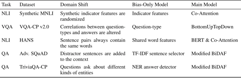
Table 1: Summary of the evaluations we perform, Domain Shift refers to what changes between the train and test data, and Bias-Only Model specifies how the bias model we use was constructed. See the main text for details.
do not further tune their hyperparameters or per-form early stopping.
We consider two extractive QA datasets, which we treat as a joint classification task where the model must select the start and end answer to-ken (Wang and Jiang, 2017). For these datasets, we build independent bias-only models for select-ing the start and end token, and separately ensem-ble those biases with the classifier’s start token and end token output distributions. We apply a ReLU layer to the question and passage embeddings, fol-lowed by max-pooling, to construct a hidden state for computing the learned-mixin weights.
We compare our methods to a reweighting base-line described below, and to training the main model without any modifications. On VQA we also compare to the adversarial methods from
Ra-makrishnan et al.(2018) and Grand and Belinkov
(2019). The other biases we consider are not based on observing only part of the input, so these adver-sarial methods cannot be directly applied.
4.1 Reweight Baseline
As a non-ensemble baseline, we train the main model on a weighted version of the data, where the weight of examplexiis1−biyi(i.e., we weigh
ex-amples by one minus the probability the bias-only model assigns the correct label). This encourages the main model to focus on examples the bias-only model gets wrong.
4.2 Hyperparameters
One of our methods (Learned-Mixin +H) requires hyperparameter tuning. However hyperparame-ter tuning is challenging in our setup since our assumption is that we have no access to out-of-domain test examples during training. A plausible option would be to tune hyperparameters on a dev
set that exhibits a related, but not identical, do-main shift to the test set, but unfortunately none of our datasets have such dev sets. Instead we follow prior work (Grand and Belinkov,2019; Ramakr-ishnan et al.,2018) and perform model selection on the test set. Although this presents an important caveat to the results of this method, we think it is still of interest to observe that the entropy regular-izer can be very impactful. Future work may be able to either construct suitable development sets, or propose other hyperparameter-tuning methods to relieve this issue. The hyperparameters selected are shown in AppendixA.
5 Experiments
We provide experiments on five different domains, summarized in Table 1, each of which requires models to overcome a challenging domain-shift between train and test data. In the following sec-tions we provide summaries of the datasets, main models and bias-only models, but leave low-level details to the appendix.
5.1 Synthetic Data
Data: We experiment with a synthetic dataset built by modifying MNLI (Bowman et al.,2015). In particular, we add a feature that is correlated with the class label to the train set, and build an out-of-domain test set by adding a randomized version of that feature to the MNLI matched dev set. We additionally construct an in-domain test set by modifying the matched dev set in the same way as was done in the train set. We build three variations of this dataset:
time the token corresponds to the example’s label (i.e., “0” if the class is “entailment”, “1” if the class is contradiction, ect.). In the out-of-domain test set, the token is selected randomly.
Excluder: The same as Indicator, but with a 3% chance the added token corresponds to the example’s label, meaning the token can usually be used to eliminate one of the three output classes.
Dependent: In the previous two settings, the added bias is independent of the example given the example’s label. To simulate a case where this independence is broken, we experiment with adding an additional feature that is correlated with the bias feature, but is not treated as being part of the bias (i.e., it is not used by the bias-only model). In particular, 80% of the time a token is added to the start of the hypothesis that matches the label with 90% probability, and the “0” token is appended to the end of the hypothesis. The other 20% of the time a random token is prepended and “1” is appended.
Bias-Only Model: The bias-only model predicts the label using the first token of the hypothesis.
Main Model: We use a recurrent co-attention model, similar to ESIM (Chen et al., 2017). De-tails are given in AppendixB.
Results: Table 2 shows the results. All ensem-bling methods work well on the Indicator bias. The reweight method performs poorly on the Ex-cluder bias, likely because the bionly model as-signs the correct class approximately 50% proba-bility for almost all the training examples, making the weights mostly uniform. This illustrates a gen-eral weakness with reweighting methods: they re-quire at least a small number of bias-free examples for the model to learn from.
The bias product method performs poorly on the Dependent bias. Inspection shows that, when the indicator is 1, the bias product model is anti-correlated with the bias. In particular, it assigns an average of22.5%probability to the class indi-cated by the bias, where an unbaised model would assign an average of 33% since the bias is ran-dom. The root cause is that, if the indicator is 1, the model knows the bias is likely to be wrong, so it learns to subtract the value the bias-only model
will produce from its own output in order to cancel out the bias-only model’s effect on the ensemble’s output.
The learned-mixin model does not suffer from this issue, and assigns the class indicated by the bias an average of 34.5% probability. Analysis shows thatg(xi)is set to0.00±0.0001when the
indicator is turned off, and to1.91±0.285 other-wise, showing that the model learns to turn off the bias-only component of the ensemble as needed, thus avoiding this over-compensating issue. The entropy regularizer appears to be unnecessary on this dataset becauseg(xi)does not go to zero.
5.2 VQA-CP
Data: We evaluate on the VQA-CP v2 (Agrawal et al.,2018) dataset, which was constructed by re-splitting the VQA 2.0 (Goyal et al.,2018) train and validation sets into new train and test sets such that the correlations between question types and answers differs between each split. For exam-ple, “tennis” is the most common answer for ques-tions that start with “What sport...” in the train set, whereas “skiing” is the most common answers for those questions in the test set. Models that choose answers because they are typical in the training data will perform poorly on this test set.
Bias-Only Model: VQA-CP comes with ques-tions annotated with one of 65 question types, cor-responding to the first few words of the question (e.g., “What color is”). The bias-only model uses this categorical label as input, and is trained on the same multi-label objective as the main model.
Main Model: We use a popular implementation3 of the BottomUpToDown (Anderson et al.,2018) VQA model. This model uses a multi-label objective, so we apply our ensemble methods by treating each possible answer as a two-class classification problem.4
Results: Table 3 shows the results. The learned-mixin method was highly effective, boosting performance on VQA-CP by about 9 points, and the entropy regularizer can increase this by another 3 points, significantly surpassing
3github.com/hengyuan-hu/bottom-up-attention-vqa
4Since the bias sometimes assigns a zero probability to
Debiasing Method Indicator Excluder Dependent
Acc. w/Bias Acc. w/Bias Acc. w/Bias
None 69.36 86.49 68.06 83.56 63.23 87.90
Reweight 75.44 82.74 70.36 83.29 69.81 85.50
Bias Product 76.27 81.32 77.33 80.41 71.85 84.98
Learned-Mixin 76.29 81.35 77.80 78.86 75.75 77.70
Learned-Mixin +H 76.77 77.65 77.90 78.57 75.79 76.65
[image:7.595.156.441.63.156.2]Unbiased Training 78.94 78.94 78.94 78.94 78.86 78.86
Table 2: Results on MNLI with different kinds of synthetic bias. The Acc columns show the accuracy on the out-of-domain test set, and the w/Bias columns show accuracy on the in-domain test. Unbiased Training is an upper bound constructed by training a model with the same randomized features that are used at test time.
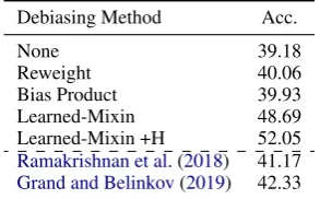
Debiasing Method Acc.
None 39.18
Reweight 40.06
Bias Product 39.93
Learned-Mixin 48.69
Learned-Mixin +H 52.05
Ramakrishnan et al.(2018) 41.17 Grand and Belinkov(2019) 42.33
Table 3: Results on the VQA-CP v2.0 test set.
prior work. For the learned-mixin ensemble, we find g(xi) is strongly correlated with the bias’s
expected accuracy5, with a spearmanr correlation of 0.77 on the test data. Qualitative examples (Figure 2) further suggest the model increases
g(xi) when it knows if can rely on the bias-only
model.
5.3 HANS
Data: We evaluate on the HANS adversarial MNLI dataset (McCoy et al.,2019). This dataset was built by constructing templated examples of entailment and non-entailment, such that the hy-pothesis sentence only includes words that are also in the premise sentence. Naively trained models tend to classify all such examples as “entailment” because detecting the presence of many shared words is an effective tactic on MNLI.
Bias-Only Model: The bias-only model is a shal-low linear classifier using the folshal-lowing features: (1) whether the hypothesis is a sub-sequence of the premise, (2) whether all words in the hy-pothesis appear in the premise, (3) the percent of words from the hypothesis that appear in the premise, (4) the average of the minimum distance between each premise word with each hypothe-sis word, measured using cosine distance with the
5
Computed asP jsijbij/
P
jbijwheresijis the score for classjon examplei
Debiasing Method Co-Attention BERT
HANS MNLI HANS MNLI
None 50.58 78.73 62.40 84.24
Reweight 52.85 77.03 69.19 83.54
Bias Product 53.69 76.63 67.92 82.97
Learned-Mixin 51.65 78.05 64.00 84.29
Learned-Mixin +H 53.35 74.50 66.15 83.97
Table 4: Accuracy on the adversarial MNLI dataset, HANS, and the MNLI matched dev set.
fasttext (Mikolov et al., 2018) word vectors, and (5) the max of those same distances. We con-strain the bias-only model to put the same amount of probability mass on the neutral and contradic-tion classes so it focuses on distinguishing entail-ment and non-entailentail-ment, and reweight the dataset so that the entailment and non-entailment exam-ples have an equal total weight to prevent a class prior from being learned.
Main Models: We experiment with both the un-cased BERT base model (Devlin et al.,2019), and the same recurrent model used for the synthetic data (see AppendixB). We use the default hyper-parameters for BERT since they work well for MNLI.
[image:7.595.108.255.221.312.2]Is this a.... ? No Question Type
Bias Answer
Higher Bias Weight
Lower Bias Weight
How many…. ? 2
How many animals? [2] G=5.61 G+=5.89
How many birds? [17] G=0.17 G+=1.95
Is this a black bear? [No] G=4.65 G+=5.96
Is this a photo or painting? [Painting]
White What color is the…. ?
G=0.87 G+=4.32
[image:8.595.75.526.63.270.2]What color is the door? [White]
What color is the tennis court? [Purple] G=0.00 G+=0.48
Pizza What kind of…. ?
What kind of food is in the box? [Pizza]
G=0.06 G+=2.93
What kind of birds are in the picture? [Seagull]
G=0.11 G+=2.34 G=0.00 G+=1.89
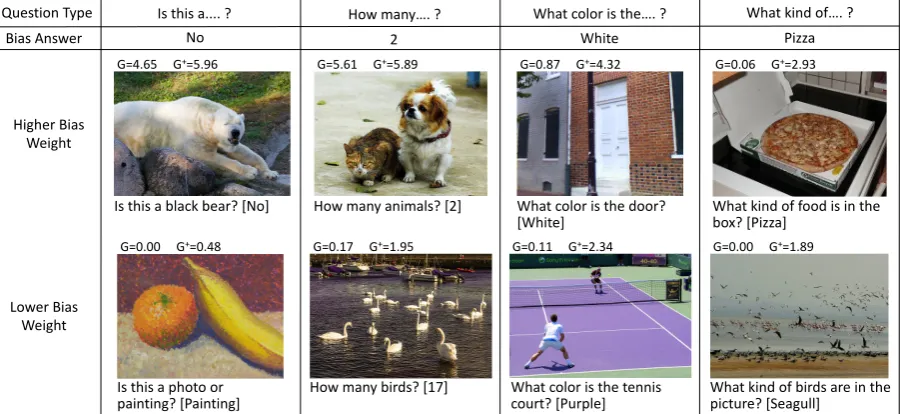
Figure 2: Qualitative examples of the values ofg(xi)on the VQA-CP training data for the learned-mixin model (labelled “G”) and learned-mixin +H model (labelled “G+”). The question type and the bias model’s highest ranked answer for that type are shown above. We findg(xi)is larger when the bias answers are likely to be correct.
5.4 Adversarial SQuAD
Data: We evaluate on the Adversarial SQuAD (Jia
and Liang, 2017) dataset, which was built by
adding distractor sentences to the passages in SQuAD (Rajpurkar et al., 2016). The sentences are built to closely resemble the question and con-tain a plausible answer candidate, but with a few key semantic changes to ensure they do not inci-dentally answer the question. Models that naively focus on sentences that contain many question words are often fooled by the new sentence.
Bias-Only Models: We consider two bias-only models: (1) TF-IDF: the TF-IDF score between each sentence and question is used to select an an-swer (meaning tokens within the same sentence all get the same score) and (2) TF-IDF Filtered: the same but excluding pronouns and numbers from the words used to compute the TF-IDF scores. The second model is motivated by the fact distractor sentences never include numbers or pronouns that occur in the question.
Main Model: We use an updated version of BiDAF (Seo et al., 2017), that uses the fasttext words vectors (Mikolov et al.,2018), includes an additional recurrent layer, and simplifies the pre-diction stage (see AppendixD).
Results: Table 5 shows the results. We find the bias product method improves performance by
up to 3 points, and the learned-mixin +H model achieves up to a 9 point gain. The importance of including the entropy penalty is explained by the fact that, without the penalty, the model learns to ignore the bias by settingsg(xi)close to zero.
For example, on the AddSent dataset with the TF-IDF filtered bias, the learned-mixin ensemble sets
g(xi) to an average of 0.13, while the
learned-mixin +H ensemble increases that to 5.16. The high values are likely caused by the fact the bias-only model is very weak, since it assigns the same score to each token in each sentence, so the model can often scale it by large values. As expected, we get better results using the TF-IDF Filtered bias which is more closely tailored to how the test set was constructed.
5.5 TriviaQA-CP
Data: We construct a changing-prior QA dataset from TriviaQA (Joshi et al., 2017) by categoriz-ing questions into three classes, Person, Location, and Other, based on what kind of entity they are asking about. During training, we hold out all the person questions or all the location questions from the train set, and evaluate on the person or location questions in the TriviaQA dev set. Details can be found in AppendixE.
Debiasing Method TF-IDF Filtered TF-IDF
AddSent AddSentOne Dev AddSent AddSentOne Dev
None 42.54 53.91 80.61 42.54 53.91 80.61
Reweight 41.55 53.06 80.59 42.74 53.83 80.51
Bias Product 47.17 57.74 78.63 44.41 55.73 78.22
Learned-Mixin 42.25 53.51 80.39 42.00 53.46 80.46
Learned-Mixin +H 51.84 60.66 75.94 48.30 58.26 74.14
Table 5: F1 scores on Adversarial SQuAD and the standard SQuAD dev set using two different bias-only models.
Debiasing Method Location Person
CP Dev CP Dev
None 41.23 59.27 39.69 55.26
Reweight 40.14 59.18 39.96 55.38
Bias Product 44.42 60.02 40.58 55.20
Learned-Mixin 41.15 61.64 41.31 56.08
Learned-Mixin +H 47.77 57.74 44.37 54.83
Table 6: EM scores on two changing priors TriviaQA datasets. The CP column shows scores on the changing priors test set, and Dev shows in-domain scores.
We only apply the model to tokens that have a NER tag, and assign all other tokens the average score given to the tokens with NER tags in order to prevent the model from reflecting a preference for entity tokens in general.
Main Model: We use a larger version of the model used for Adversarial SQuAD (see AppendixD), to account for the larger dataset.
Results: Table6shows the results. Similar to ad-versarial SQuAD, the bias product method is mod-erately effective, and the ensemble method is su-perior as long as a suitable regularizer is applied. We again observe that the learned-mixin method tends to pushg(xi) close to zero without the
en-tropy penalty (average of0.25without the penalty vs.5.01with the penalty on the Location dev set). We see smaller gains on the person dataset. One possible cause is that differentiating between peo-ple and other named entities, such as organizations or groups, is difficult for the main model, and as a result it does not learn a strong non-person prior even without the use of a debiasing method.
5.6 Discussion
Despite tackling a diverse range of problems, we were able to improve out-of-domain performance in all settings. The bias product method works consistently, but can almost always be signifi-cantly out-performed by the learned-mixin method
with an appropriate entropy penalty. The reweight baseline improved performance on HANS, but was relatively ineffective in other cases.
Increasing the out-of-domain performance usu-ally comes at the cost of losing some in-domain performance, which is unsurprising since the bi-ased approaches we are removing are helpful on the in-domain data. TriviaQA-CP stands out as a case where this trade-off is minimal.
A possible issue is that our methods reduce the need for the model to solve examples the bias-only model works well on (since the ensemble’s predic-tion will already be mostly correct for those ex-amples), which effectively reduces the amount of training data. An ideal approach would be to block the model from using the bias-only method, and require it to solve examples the bias-only method solves through other means. We suspect this will necessitate a more clear-box method since it re-quires doing fine-grained regularization of how the model is solving individual examples.
6 Conclusion
Our key contribution is a method of using human knowledge about what methods will not generalize well to improve model robustness to domain-shift. Our approach is to train a robust model in an en-semble with a pre-trained naive model, and then use the robust model alone at test time. Extensive experiments show that our method works well on two adversarial datasets, and two changing-prior datasets, including a 12 point gain on VQA-CP. Future work includes learning to automatically de-tect dataset bias, which would allow our method to be applicable with less specific prior knowledge.
Acknowledgements
References
Aishwarya Agrawal, Dhruv Batra, Devi Parikh, and Aniruddha Kembhavi. 2018. Don’t Just Assume; Look and Answer: Overcoming Priors for Visual Question Answering. InCVPR.
Ankesh Anand, Eugene Belilovsky, Kyle Kastner, Hugo Larochelle, and Aaron Courville. 2018. Blindfold Baselines for Embodied QA. Computing
Research Repository, arXiv:1811.05013. Version 1.
Peter Anderson, Xiaodong He, Chris Buehler, Damien Teney, Mark Johnson, Stephen Gould, and Lei Zhang. 2018. Bottom-Up and Top-Down Attention for Image Captioning and Visual Question Answer-ing. InCVPR.
Stanislaw Antol, Aishwarya Agrawal, Jiasen Lu, Mar-garet Mitchell, Dhruv Batra, C Lawrence Zitnick, and Devi Parikh. 2015. VQA: Visual Question An-swering. InICCV.
Dzmitry Bahdanau, Kyunghyun Cho, and Yoshua Ben-gio. 2015. Neural Machine Translation by Jointly Learning to Align and Translate. InICLR.
Yonatan Belinkov and Yonatan Bisk. 2018. Syn-thetic and Natural Noise Both Break Neural Ma-chine Translation. InICLR.
Yonatan Belinkov, Adam Poliak, Stuart M Shieber, Benjamin Van Durme, and Alexander M Rush. 2019. On Adversarial Removal of Hypothesis-only Bias in Natural Language Inference. InStarSem.
Samuel R Bowman, Gabor Angeli, Christopher Potts, and Christopher D Manning. 2015. A Large Anno-tated Corpus for Learning Natural Language Infer-ence. InEMNLP.
Kaylee Burns, Lisa Anne Hendricks, Kate Saenko, Trevor Darrell, and Anna Rohrbach. 2018. Women Also Snowboard: Overcoming Bias in Captioning Models. InECCV.
Ozan Caglayan, Pranava Madhyastha, Lucia Specia, and Lo¨ıc Barrault. 2019. Probing the Need for Vi-sual Context in Multimodal Machine Translation. In
NAACL.
Nicholas Carlini and David Wagner. 2018. Audio Ad-versarial Examples: Targeted Attacks on Speech-to-Text. In 2018 IEEE Security and Privacy Work-shops.
Jifan Chen and Greg Durrett. 2019. Understanding Dataset Design Choices for Multi-hop Reasoning.
InNAACL.
Qian Chen, Xiaodan Zhu, Zhenhua Ling, Si Wei, Hui Jiang, and Diana Inkpen. 2017. Enhanced LSTM for Natural Language Inference. InACL.
Eunsol Choi, He He, Mohit Iyyer, Mark Yatskar, Wen-tau Yih, Yejin Choi, Percy Liang, and Luke Zettle-moyer. 2018. QuAC: Question Answering in Con-text. InEMNLP.
Christopher Clark and Matt Gardner. 2018.Simple and Effective Multi-Paragraph Reading Comprehension. InACL.
Peter Clark, Isaac Cowhey, Oren Etzioni, Tushar Khot, Ashish Sabharwal, Carissa Schoenick, and Oyvind Tafjord. 2018. Think you have Solved Question An-swering? Try ARC, the AI2 Reasoning Challenge.
Computing Research Repository, arXiv:1803.05457.
Version 1.
Peter Clark, Oren Etzioni, Tushar Khot, Ashish Sab-harwal, Oyvind Tafjord, Peter Turney, and Daniel Khashabi. 2016. Combining Retrieval, Statistics, and Inference to Answer Elementary Science Ques-tions. InAAAI.
Jacob Devlin, Ming-Wei Chang, Kenton Lee, and Kristina Toutanova. 2019. BERT: Pre-training of Deep Bidirectional Transformers for Language Un-derstanding. InNAACL.
Harrison Edwards and Amos Storkey. 2016. Censoring Representations with an Adversary. InICLR.
Shi Feng, Eric Wallace, and Jordan Boyd-Graber. 2019. Misleading Failures of Partial-input Baselines. In
ACL.
Jenny Rose Finkel, Trond Grenager, and Christopher Manning. 2005. Incorporating Non-local Informa-tion into InformaInforma-tion ExtracInforma-tion Systems by Gibbs Sampling. InACL.
Max Glockner, Vered Shwartz, and Yoav Goldberg. 2018. Breaking NLI Systems with Sentences that Require Simple Lexical Inferences. InACL.
Yash Goyal, Tejas Khot, Douglas Summers-Stay, Dhruv Batra, and Devi Parikh. 2018. Making the V in VQA Matter: Elevating the Role of Image Un-derstanding in Visual Question Answering.IJCV.
Gabriel Grand and Yonatan Belinkov. 2019. Adversar-ial Regularization for Visual Question Answering: Strengths, Shortcomings, and Side Effects. In Pro-ceedings of the Second Workshop on Shortcomings in Vision and Language.
Suchin Gururangan, Swabha Swayamdipta, Omer Levy, Roy Schwartz, Samuel R Bowman, and Noah A Smith. 2018. Annotation Artifacts in Natu-ral Language Inference Data. InNAACL.
He He, Sheng Zha, and Haohan Wang. 2019. Unlearn Dataset Bias in Natural Language Inference by Fit-ting the Residual. Computing Research Repository, arXiv:1908.10763. Version 1.
Geoffrey E. Hinton. 2002. Training Products of Ex-perts by Minimizing Contrastive Divergence. Neu-ral Computation.
Robin Jia and Percy Liang. 2017. Adversarial Ex-amples for Evaluating Reading Comprehension Sys-tems. InEMNLP.
Mandar Joshi, Eunsol Choi, Daniel S Weld, and Luke Zettlemoyer. 2017. TriviaQA: A Large Scale Dis-tantly Supervised Challenge Dataset for Reading Comprehension. InACL.
Byungju Kim, Hyunwoo Kim, Kyungsu Kim, Sungjin Kim, and Junmo Kim. 2019. Learning Not to Learn: Training Deep Neural Networks with Biased Data. InCVPR.
Diederik P Kingma and Jimmy Ba. 2015. Adam: A Method for Stochastic Optimization. InICLR.
Mike Lewis and Angela Fan. 2019. Generative Ques-tion Answering: Learning to Answer the Whole Question. InICLR.
Tom McCoy, Ellie Pavlick, and Tal Linzen. 2019. Right for the Wrong Reasons: Diagnosing Syntactic Heuristics in Natural Language Inference. InACL.
Tomas Mikolov, Edouard Grave, Piotr Bojanowski, Christian Puhrsch, and Armand Joulin. 2018. Ad-vances in Pre-Training Distributed Word Represen-tations. InLREC.
Sewon Min, Eric Wallace, Sameer Singh, Matt Gard-ner, Hannaneh Hajishirzi, and Luke Zettlemoyer. 2019. Compositional Questions Do Not Necessitate Multi-hop Reasoning. InACL.
Pranav Rajpurkar, Jian Zhang, Konstantin Lopyrev, and Percy Liang. 2016. SQuAD: 100, 000+ Questions for Machine Comprehension of Text. InEMNLP.
Sainandan Ramakrishnan, Aishwarya Agrawal, and Stefan Lee. 2018. Overcoming Language Priors in Visual Question Answering with Adversarial Regu-larization. InNeurIPS.
Siva Reddy, Danqi Chen, and Christopher D. Manning. 2019. CoQA: A Conversational Question Answer-ing Challenge. InTACL.
Roy Schwartz, Maarten Sap, Ioannis Konstas, Li Zilles, Yejin Choi, and Noah A Smith. 2017. The Effect of Different Writing Tasks on Linguistic Style: A Case Study of the ROC Story Cloze Task. InCoNLL.
Minjoon Seo, Aniruddha Kembhavi, Ali Farhadi, and Hannaneh Hajishirzi. 2017. BiDirectional Attention Flow for Machine Comprehension. InICLR.
Andrew Smith, Trevor Cohn, and Miles Osborne. 2005. Logarithmic Opinion Pools for Conditional Random Fields. InACL.
Rupesh Kumar Srivastava, Klaus Greff, and J¨urgen Schmidhuber. 2015. Highway networks. In Deep
Learning Workshop (ICML).
Fabian M Suchanek, Gjergji Kasneci, and Gerhard Weikum. 2007. Yago: A Core of Semantic Knowl-edge. InWWW.
Christian Szegedy, Wojciech Zaremba, Ilya Sutskever, Joan Bruna, Dumitru Erhan, Ian Goodfellow, and Rob Fergus. 2014. Intriguing Properties of Neural Networks. InICLR.
Shuohang Wang and Jing Jiang. 2017. Machine Comprehension Using Match-LSTM and Answer Pointer. InICLR.
Tianlu Wang, Jieyu Zhao, Kai-Wei Chang, Mark Yatskar, and Vicente Ordonez. 2018. Adversar-ial Removal of Gender from Deep Image Rep-resentations. Computing Research Repository, arXiv:1811.08489. Version 2.
Yicheng Wang and Mohit Bansal. 2018. Robust Ma-chine Comprehension Models via Adversarial Train-ing. InNAACL.
Johannes Welbl, Pontus Stenetorp, and Sebastian Riedel. 2018. Constructing Datasets for Multi-hop Reading Comprehension across Documents.TACL.
Zhilin Yang, Peng Qi, Saizheng Zhang, Yoshua Ben-gio, William W Cohen, Ruslan Salakhutdinov, and Christopher D Manning. 2018.Hotpotqa: A Dataset for Diverse, Explainable Multi-hop Question An-swering. InEMNLP.
Rowan Zellers, Yonatan Bisk, Roy Schwartz, and Yejin Choi. 2018. Swag: A Large-Scale Adversarial Dataset for Grounded Commonsense Inference. In
EMNLP.
Brian Hu Zhang, Blake Lemoine, and Margaret Mitchell. 2018a. Mitigating Unwanted Biases with Adversarial Learning. InAIES.
Peng Zhang, Yash Goyal, Douglas Summers-Stay, Dhruv Batra, and Devi Parikh. 2016. Yin and Yang: Balancing and Answering Binary Visual Questions. InCVPR.
Sheng Zhang, Xiaodong Liu, Jingjing Liu, Jianfeng Gao, Kevin Duh, and Benjamin Van Durme. 2018b. ReCoRD: Bridging the Gap between Human and Machine Commonsense Reading Comprehension.
Computing Research Repository, arXiv:1810.12885.
Version 1.
Jieyu Zhao, Tianlu Wang, Mark Yatskar, Vicente Or-donez, and Kai-Wei Chang. 2017. Men Also Like Shopping: Reducing Gender Bias Amplification us-ing Corpus-level Constraints. InEMNLP.
A Entropy Penalty Weights
Dataset Experiment Penalty
Synthetic Indicator 0.01
Synthetic Excluder 0.005
Synthetic Dependent 0.005
VQA-CP - 0.36
HANS Recurrent 0.03
HANS BERT 0.03
Adver. SQuAD TF-IDF Filtered 2.0
Adver. SQuAD TF-IDF 2.0
TriviaQA-CP Location 0.4
[image:12.595.79.286.62.211.2]TriviaQA-CP Person 0.2
Table 7: Entropy penalty weight for the learned-mixin +H ensemble on all our experiments.
B Co-Attention NLI Model
The model we use for NLI is based on ESIM (Chen et al., 2017). It has the follow-ing stages:
Embed: Embed the words using a character CNN, following what was done by Seo et al.
(2017), and the fasttext crawl word embed-dings (Mikolov et al., 2018), then run a shared BiLSTM over the results.
Co-Attention: Compute an attention matrix using the formulation from Seo et al. (2017), and use it to compute a context vector for each premise word (Bahdanau et al.,2015). Then build an augmented vector for each premise word by concatenating the word’s embedding, the context vector, and the elementwise product of the two. Augmented vectors for the hypothesis are built in the same way using the transpose of the attention matrix.
Pool: Run another shared BiLSTM over the augmented vectors, and max-pool the results. The max-pooled vectors from the premise and hypothesis are fed into a fully-connected layer, and then into a softmax layer with three outputs to compute class probabilities.
We apply variational dropout at a rate of 0.2 between all layers, and to the recurrent states of the LSTM, and train the model for 30 epochs using the Adam optimizer (Kingma and Ba,2015) with a batch size of 32. The learning rate is decayed by 0.999 every 100 steps. We use 200 dimensional LSTMs and a 50 dimensional fully
connected layer.
C Fine-Grained HANS Results
We show the scores our methods achieve for the various heuristics used in HANS in Table 8. Our methods reduce the extent to which models naively guess entailment in all cases. Interest-ingly, the BERT model shows significantly de-graded performance on the entailment examples when using the reweight and bias product method, but largely maintains its performance on those ex-amples when using the learned-mixin method.
D Modified BiDAF QA Model
The model we use for QA is based on BiDAF (Seo et al.,2017). It has the following stages:
Embed: Embed the words using a character CNN followingSeo et al.(2017) and the fasttext crawl word embeddings (Mikolov et al., 2018). Then run a BiLSTM over the results to get context-aware question embeddings and passage embeddings.
Bi-Attention: Apply the bi-directional atten-tion mechanism fromSeo et al.(2017) to produce question-aware passage embeddings.
Predict: Apply a fully connected layer, then two more BiLSTM layers, then a two dimensional linear layer to produce start and end scores for each token.
We apply variational dropout at a rate of 0.2 between all layers. We use the Adam opti-mizer (Kingma and Ba, 2015) with a batch size of 45, while decaying the learning rate by 0.999 every 100 steps.
For SQuAD, we use a 200 dimensional fully connected layer and 100 dimensional LSTMs.
For TriviaQA we use a 256 dimensional fully connected layer and 128 dimensional LSTMs, with highway connections between each BiL-STM (Srivastava et al., 2015) and a recurrent dropout rate of 0.2.
E TriviaQA-CP
In this section we discuss our changing-prior Triv-iaQA dataset, TrivTriv-iaQA-CP. This dataset was built by training a classifier to identify TriviaQA (Joshi
Model Debiasing Method MNLI Correct:Entailment Correct:Non-entailment
Lexical Subseq. Const Lexical Subseq. Const
Co-Attention
None 78.73 97.83 99.67 97.28 1.37 3.68 3.68
Reweight 77.03 80.10 77.84 73.76 15.68 34.27 35.44
Bias Product 76.63 77.89 76.61 70.95 17.89 35.11 43.71
Learned-Mixin 78.05 94.84 97.25 91.19 3.69 9.57 13.37
Learned-Mixin +H 74.50 67.18 61.05 47.13 27.41 56.82 60.53
BERT
None 84.24 96.30 99.58 99.30 49.03 7.88 22.30
Reweight 83.54 67.93 84.34 80.97 77.44 44.87 59.57
Bias Product 82.97 53.67 69.47 70.88 81.34 62.93 69.23
Learned-Mixin 84.29 95.64 99.52 99.14 55.41 8.34 25.96
[image:13.595.101.501.64.199.2]Learned-Mixin +H 83.97 91.98 98.20 97.98 64.99 13.25 30.48
Table 8: Scores on individual heuristics in HANS, with scores on the MNLI matched dev set for reference. Results are an average of 8 runs.
Statistic Location Person
Num Train 60,133 52,953
Num Test 1,992 2,865
Avg. Passage Length 318 317
Avg. Question Length 16.7 16.0
Table 9: Statistics for the TriviaQA-CP datasets.
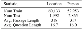
locations, or other topics, and then selecting an answer-containing passage for each question as context. There are two versions of this dataset: a person changing-priors dataset that was built by removing the person questions from the train set and using only person questions from the dev set for evaluation, and a location changing-priors dataset that was built by repeating this process for location questions. Statistics for these two sets are shown in Table 9. We review the three-step procedure we used to construct this dataset below.
Distantly Supervised Classification: We first train a preliminary question-type classifier using distant supervision. We noisily label person and location questions using a manually con-structed set of patterns (e.g., questions with the phrase “What is the family name of...” are almost always about people), and by attempting to look up the answers in the Yago database (Suchanek et al.,2007) and checking if the answer belongs to a person or location category. Questions that did not match either of these heuristics are labelled as other.
We use these labels to train a simple recurrent model that embeds the question using the fasttext words vectors, applies a 100 dimensional BiL-STM, max-pools, and then applies a softmax layer with 3 outputs. We train the model for 3 epochs using the Adam optimizer (Kingma and Ba,
2015), and apply 0.5 dropout to the embeddings and 0.2 dropout to the recurrent states and the output of the max-pooling layer.
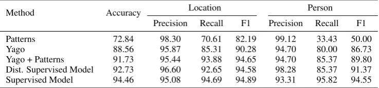
Supervised Classification: Next we use higher quality labels to train a second linear classifier to re-calibrate the recurrent model’s predictions, and to integrate its predictions with the distantly supervised heuristics. An author manually labelled 1,100 questions, then a classifier was trained on those questions using the predictions from the recurrent model as features, as well as two additional features built from looking up the category of the answer in Yago as before. This classifier was then used to decide the final question classifications.
Table10shows the accuracy of these classifiers. The final model achieves about 95% accuracy. We find about 25% of the questions are about people and about 20% of the questions are about locations.
Paragraph Selection: In TriviaQA, each question is paired with multiple documents. We simplify the task by selecting a single answer-containing paragraph for each question. We use the approach
of Clark and Gardner (2018) to break up the
[image:13.595.93.268.254.316.2]Method Accuracy Location Person
Precision Recall F1 Precision Recall F1
Patterns 72.84 98.30 70.61 82.19 99.12 33.43 50.00
Yago 88.56 95.87 85.31 90.28 94.70 80.00 86.73
Yago + Patterns 91.73 95.44 93.88 94.65 94.70 85.37 89.80
Dist. Supervised Model 92.73 96.60 92.65 94.58 98.28 85.37 91.37
[image:14.595.115.484.353.439.2]Supervised Model 94.46 95.08 94.69 94.89 93.31 95.82 94.55