Battery Aware Mobile Relay for
Wireless Sensor Network
Noritaka Shigei
∗, Issei Fukuyama
∗†, Hiromi Miyajima
∗‡, and Yogi Anggun Saloko Yudo
§Abstract—Multi-hop communication is used for prolonging the lifetime of WSN (Wireless Sensor Network). In recent years, mobile relay has been studied. The concept of mobile relay is that the mobile nodes change their locations so as to minimize the total energy consumed by both wireless transmission and locomotion. The conventional methods, however, do not take into account the remaining energy on mobile nodes, and as a result they do not always prolong the network lifetime. In this study, we propose two types of algorithms for mobile relay. The proposed algorithms take into account the battery level and overlapping multiple data flows. We show their effectiveness by simulation.
Index Terms—mobile sensor node, wireless sensor network, multi-hop communication, network lifetime, battery aware
I. INTRODUCTION
T
He wireless sensor network (WSN) is a key component for ubiquitous computing[1]. A WSN consists of a num-ber of sensor nodes. Each sensor node senses environmental conditions such as temperature, pressure and light, and it sends the sensed data to a sink node or a base station, which is a long way off in general. Since the sensor nodes are powered by limited power batteries, in order to prolong the life time of the network, low energy consumption is important for sensor nodes. In general, radio communication consumes the most amount of energy, which is proportional to the data size and proportional to the square or the fourth power of the distance.Thanks to the advance in mobile sensor platform tech-nology, in recent years, it has been taken into attention that mobile elements are utilized to improve the WSN’s performances[2] such as coverage[3], connectivity[4], reliability[5] and energy efficiency[6], [7]. Mobile relay has been studied in order to reduce the energy consumption in WSNs[8], [9]. The concept of mobile relay is that the mobile nodes change their locations so as to minimize the total energy consumed by both wireless transmission and locomotion. The conventional methods, however, do not take into account the battery level, and as a result they do not always prolong the network lifetime.
In this paper, we propose two types of algorithms for mobile relay. The proposed algorithms take into account the remaining energy on mobile nodes. Firstly the algorithm is presented for single data flow case, and them the algorithm is extended to the case of multiple data flows. Our simulation results show that, compared with the conventional methods, both algorithms are superior in terms of prolonging the
* Graduate School of Science and Engineering, Kagoshima University, 1-21-40 Korimoto, Kagoshima 890-0065, Japan (corresponding author N. Shigei to provide email: [email protected])
†email: [email protected] ‡email: [email protected]
§PT. Telekomunikasi Indonesia Tbk, Indonesia, (email: [email protected])
network lifetime and the algorithm for multiple data flows is the most effective.
II. MOBILEWSN MODEL
In this paper, we consider a similar WSN model as in [8], [9]. The network consists of N mobile nodes. The mobile node is assumed to have the following functions and fea-tures: 1) sensing environmental factors such as temperature, pressure and light, 2) data processing by low-power micro-controller, 3) a radio communication function in which the transmission power is controlled according to the distance to the target node, 4) powered by a limited life battery, 5) their own location can be estimated by an equipped GPS unit or other system, and 6) movable by an equipped electric motor. The energy consumption model is as follows. When a mobile node moves a distance of d [m], it consumes the following energy
EM(d) =k·d [J], (1)
where the parameterk[J/m] depends on the mobile platform and the moving velocity. When a node transmits a data of
m[bit] over a distance of d[m], it consumes the following energy
ET(d, m) =m(a+b·d2) [J], (2) where the parameters a and b depend on the environment and the radio platform. Further, when a node receives a data ofm [bit], it consumes the following energy
ER(m) =c·m [J], (3)
where the parameterc depends on the radio platform. The considered WSN operates as follows: One or multiple nodes of N mobile nodes act as source nodes, and the source nodes send their sensing date to a sink node. The sensing data is transferred through one or multiple hops. Whether it uses direct or multi-hop transmission depends on their transmission costs. For example, let the distances between source and sink, source and relay, and sink and relay be denoted byd1,d2andd3, respectively. If the direct transmission cost of ET(d1, m) is larger than the multi-hop one of ET(d2, m) + ET(d3, m), then the multi-hop transmission via the relay node is used.
III. MOBILERELAY
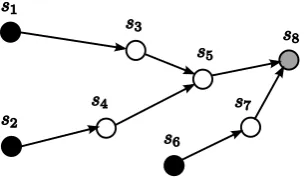
Fig. 1. An example of directed tree for multiple data flows: source (leaf) nodes ares1,s2ands6, sink node iss8,S(s5) ={s3, s4}, andD(s5) =
[image:2.595.320.540.57.222.2]{s1, s2}.
Fig. 2. An example of directed tree for single data flow:s1 is the source
(leaf) node ands4is the sink (root) node.
N nodes in the network. Letoibe the initial position of node
si for1≤i≤N andO= (o1,· · ·, oN)be its list. LetSsrc
be the subset of S representing the source nodes. Letssnk be the single sink in S. Let E be the set of directed arcs
(si, sj) in the directed tree in which each source node is a leaf and the sink node is the root. An example of the directed tree is shown in Fig.1. Let mi be the total number of bits to be transmitted by node si for 1 ≤i≤N. Let ui be the position of node si for 1 ≤i≤N and U = (u1,· · ·, uN) be its list. The transmission cost for a formationU is given by the following equation.
c(U) = ∑
(si,sj)∈E
a·mi+b||ui−uj||2mi+k||oi−ui|| (4)
Given instances ofS,O,Ssrc,ssnkandE, then the problem is to determine the mobile node formation U so as to minimize the transmission costC(U).
An optimal solution for the problem can be determined by an iterative algorithm. Let us explain the algorithm for single data flow case where the number of source nodes is one. Note that the directed tree for single data flow is a path from the source to the root as shown in Fig.2. We assume thatSsrc={s1},ssnk=sn and the relaying order iss1,s2,
s3,· · ·. Letuti= (xit, yti)be the position of nodesiaftert-th
iteration (t≥0), where u0
i =oi. In the iterative algorithm, the updatation of positions alternates between odd number and even number nodes. If t is odd number, for all 1 ≤ j ≤n/2, each odd-numbered node s2j−1 calculates a new position as ut
2j−1 and each even-numbered node s2j keeps its position, that is ut
2j =u t−1
2j . Otherwise, vice versa. As the iterationt increases, the formation of nodes approaches to the optimal one. Note that, at each iteration, the mobile nodes do not actually move and just calculate the positions.
The new position ut
i of node si at t-th iteration is de-rived from the cost function on the node positions Ut =
(ut
1,· · ·, utn). At t-th iteration, the energy consumption of
nodesi is as follows.
ci(Ut) =k||uti−oi||+m(a+b||uti+1−u t i||
2
) (5)
20 30 40 50 60 70 80 90
0 20 40 60 80 100 120 140 160 Initial position
After 2nd iteration After 4th iteration After 6th iteration After 8th iteration
Fig. 3. An example of the position change at each iteration form= 40MB,
k= 2.0J/m,a= 0.6×10⁻⁷ J/bit andb= 4.0×10⁻¹⁰Jm−2/bit.
Since uti−1 anduti+1 are fixed, the cost function for deter-mining the optimal positionuti is as follows.
Ci(Ut) =ci(Ut) +m(a+b||uti−u t i−1||
2) (6) The optimal position is obtained by solving the equations
∂Ci(Ut)
∂xt i
= 0 and ∂Ci(Ut)
∂yt i
= 0 as follows. When xti−1 + xti+1≥2xti,
xti =1 2(x
t i−1+x
t i+1)−Y
t
i, (7)
where
Yit= k 4b·m·
1 √
1 + (y
t i−1+y
t i+1−2qi)2
(xt i−1+x
t i+1−2pi)2
(8)
Otherwise,
xti =1 2(x
t i−1+x
t i+1) +Y
t
i. (9)
For any case,
yit=
yti−1+yti+1−2qi
xt
i−1+xti+1−2pi
(xti−pi) +qi. (10)
Since the above calculations forsi do not need any informa-tion on other nodes than itselfsi and its neighboring nodes
si−1, si+1, the iterative algorithm can be decentrally per-formed by each individual node with information exchange between neighboring nodes.
The number of iterations for convergence needed for convergence to the optimal position depends on the initial formation and the used parameters such as m, a, b andk. However, for most typical cases, the number of iterations around 10 provides a good convergence. Fig.3 is an example of the position change at each iteration for a typical setting. The algorithm can be extended to the case of multiple data flows where the number of source nodes is more than one. An example of the directed tree for this case is shown in Fig.1. Let S(si) be the set of Si’s child nodes in the directed tree. Let D(si) be the set of nodes that are leafs and si’s grandchildren. Let Di be the number of nodes in
[image:2.595.303.548.375.562.2]parent node ofsiin the directed tree. Then the cost function is as follows.
Ci(Ut) =kkuti−oik+Dim(a+bkutd−u t ik
2)
+ ∑
sl∈S(si)
Dlm(a+bkuti−u t lk
2) (11)
The optimal position can be obtained by solving the equa-tions ∂Ci(Ut)
∂xt i
= 0 and ∂Ci(Ut)
∂yt i
= 0.
IV. BATTERYAWAREMOBILERELAY
In this section, we propose battery aware algorithms for mobile relay. The aim of the proposed approach is to maximize the network lifetime define as the time where all the nodes are alive. This approach has the following advantages: 1) The path reconfiguration needed in the case of node down on the transmission path can be avoidable as much as possible, and 2) the coverage of sensing area by mobile nodes can be kept high. The proposed algorithms determine the node configuration such that a relay node with lower remaining energy consumes less energy and a relay node with higher remaining energy supports lower energy nodes by consuming more energy.
A. Battery Aware Mobile Relay for Single Data Flow
In this subsection, we explain the algorithm for single data flow case where the number of source nodes is one, that is
Ssrc={s1} andssnk=sn. We assume that the relay order
iss1,s2,s3,· · ·. Letei be the battery energy level of node
si. The proposed cost function is as follows:
Ci(Ut) =
k||ut i−oi||
ei
+m(a+b||u
t i+1−u
t i||
2)
ei
+m(a+b||u
t i−u
t i−1||
2)
ei−1
(12)
As ei decreases, the first and second terms in the cost function keep the movement and transmission ranges of node
sismaller. Asei−1decreases, the third term encourages node
sito offer more assistance to nodesi−1. The optimal position is obtained by solving the equations ∂Ci(Ut)
∂xt i
= 0 and ∂Ci(Ut)
∂yt i
= 0as described in Section III. Whenxti−1+xti+1≥ 2xti,
xti= eix
t
i−1+ei−1xti+1
ei+ei−1
−Yit, (13)
where
Yit=
ei−1k
2bm(ei+ei+1)·
1 √
1 + (ei(y
t
i−1−qi)+ei−1(yti+1−qi))2
(ei(xti−1−pi)+ei−1(xti+1−pi))2
(14) Otherwise,
xti= eix
t
i−1+ei−1xti+1
ei+ei−1
+Yit. (15)
For any case,
yti = ei(y
t
i−1−qi) +ei−1(yti+1−qi)
ei(xti−1−pi) +ei−1(xti+1−pi)
(xti−pi) +qi. (16)
The above calculations forsi, as well as Eqs.(7)∼(10), do not need any information on other nodes than itself si and
its neighboring nodessi−1si+1. Therefore, its iterative algo-rithm can be also decentrally performed by each individual node with information exchange between neighboring nodes.
B. Battery Aware Mobile Relay for Multiple Data Flows
In this subsection, we extend the proposed algorithm to the case of multiple data flows. Let S(si) be the set of nodes that send the data directly tosion the data flows. LetD(si) be the set of source nodes whose transmitting data is relayed by nodesi. LetDi be the number of nodes in D(si). For a given nodesi, let sd be the node that is the parent node of
si in the directed tree. Then the cost function is as follows.
Ci(Ut) =
kkuti−oik
ei
+Dim(a+bku
t d−u
t ik
2)
ei
+ ∑
sl∈S(si)
Dlm(a+bkuti−utlk2)
el
(17)
The optimal position is also obtained by solving the equa-tions ∂Ci(Ut)
∂xt i
= 0 and ∂Ci(Ut)
∂yt i
= 0. When xti−1+xti+1 ≥ 2xti,
xti= Dix
t d+ei
∑
sl∈S(si)
Dl
elx
t l
Di+ei
∑
sl∈S(si)
Dl
el
−Yit, (18)
where
Yit= k
2bm (
Di+ei
∑
sl∈S(si)
Dl el )× 1 + (
Di(ytd−qi) +ei
∑
sl∈S(si)
Dl
el(y
t l−qi)
Di(xtd−pi) +ei
∑
sl∈S(si)
Dl
el(x
t l−pi)
)2
−1/2
.
(19)
Otherwise,
xti= Dix
t d+ei
∑
sl∈S(si)
Dl
elx
t l
Di+ei
∑
sl∈S(si)
Dl
el
+Yit. (20)
For any case,
yit= Di(y
t
d−qi) +ei
∑
sl∈S(si)
Dl
el(y
t l−qi)
Di(xtd−pi) +ei
∑
sl∈S(si)
Dl
el(x
t l−pi)
(xti−pi)
+qi. (21)
The iterative algorithm with the above equations can be also decentrally performed by each individual node with information exchange between neighboring nodes.
V. NUMERICALSIMULATION
In order to the effectiveness of the proposed methods, we perform numerical simulations. In the simulation,N mobile sensor nodes are initially randomly distributed in a 150m× 150 square field. From theN nodes,10∼30source nodes and one sink node are randomly selected. The parameter setting used for energy model is as follows: k = 2 J/m,
a = 0.6 ×10⁻⁷ J/bit, b = 4.0×10⁻¹⁰ Jm−2/bit and
0 20 40 60 80 100 120 140 160
0 20 40 60 80 100 120 140 160
y [m]
x [m]
[image:4.595.62.363.47.649.2]Sink Route 1 Route 2 Route 3 Route 4 Route 5 Route 6 Route 7 Route 8 Route 9 Route 10
Fig. 4. An initial configuration.
0 20 40 60 80 100 120 140 160
0 20 40 60 80 100 120 140 160
y [m]
x [m]
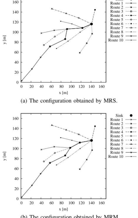
Sink Route 1 Route 2 Route 3 Route 4 Route 5 Route 6 Route 7 Route 8 Route 9 Route 10
(a) The configuration obtained by MRS.
0 20 40 60 80 100 120 140 160
0 20 40 60 80 100 120 140 160
y [m]
x [m]
Sink Route 1 Route 2 Route 3 Route 4 Route 5 Route 6 Route 7 Route 8 Route 9 Route 10
(b) The configuration obtained by MRM.
Fig. 5. The configurations obtained by the conventional methods MRS and MRM for an initial configuration shown in Fig.4
charged in the range of 10 kJ∼150 kJ. We assume that the sink node uses an unlimited energy source.
We evaluate the following four types of MR (Mobile Relay configuration) methods.
• MR for Single data flow (MRS) renews only the positions of the nodes having just one child node in
0 20 40 60 80 100 120 140 160
0 20 40 60 80 100 120 140 160
y [m]
x [m]
Sink Route 1 Route 2 Route 3 Route 4 Route 5 Route 6 Route 7 Route 8 Route 9 Route 10
(a) The configuration obtained by BMRS.
0 20 40 60 80 100 120 140 160
0 20 40 60 80 100 120 140 160
y [m]
x [m]
Sink Route 1 Route 2 Route 3 Route 4 Route 5 Route 6 Route 7 Route 8 Route 9 Route 10
[image:4.595.314.540.58.430.2](b) The configuration obtained by BMRM.
Fig. 6. The configurations obtained by the proposed methods BMRS and BMRM for an initial configuration shown in Fig.4
the directed tree by using Eqs.(7), (8), (9) and (10), and it does not change the initial positions for the nodes having more than one child nodes.
• MR for Multiple data flows (MRM) renews the positions of the nodes having more than one child node in the directed tree by using the equations based on Eq.(11), and it also renews the other nodes by using Eqs.(7), (8), (9) and (10).
• Battery aware MR for Single data flow (BMRS)
renews the positions of the nodes having just one child node in the directed tree by using Eqs.(13), (14), (15) and (16), and it does not change the initial positions for the nodes having more than one child nodes.
• Battery aware MR for Multiple data flow (BMRM)
renews the positions of the nodes having more than one child node in the directed tree by using Eqs.(18), (19), (20) and (21), and it also renews the other nodes by using Eqs.(13), (14), (15) and (16).
[image:4.595.50.285.281.651.2]Figures 5 and 6 show the configurations obtained by MRS, MRM, BMRS and BMRM for the initial configuration shown in Fig.4. From the result, we can observe the following tendencies.
• For MRS and MRM (Figs. 5.(a) and 5.(b)), the lengths of edges are almost same in each of paths that are subgraph of the directed tree and whose internal node have just one child and one parent.
• The paths for MRM are straight compared with the ones for MRS. This is because the nodes having more than one child move toward their optimal positions.
• For BMRS and BMRM (Figs. 6.(a) and 6.(b)), the paths become near straight compared with the original formation. However, the length of edges are obviously different. This is because the child node of a short edge has less remaining energy.
• BMRM provides more shorter paths than BMRS, be-cause the nodes having more than one child move toward their optimal positions.
Next, the methods are evaluated in terms of the amount of data that the source node collects until any node goes down due to battery dead. The simulation results for the numbers of source nodes 10, 20 and 30 are shown in Figure 7. The improvement ratio is defined as follows:
B
A ×100 [%], (22)
where B is the amount of data collected for each of the methods and A is the amount of data collected for the initial node formation. The results are average values for 100 instances of the network model.
From the results shown in Fig.7, we can observe the following tendencies.
(1) When the chunk size is more than about 30MB, all the methods provides constant improvement.
(2) The methods moving the all node positions such as MRM and BMRM are more effective than the methods only moving the nodes on single data flow such as MRS and BMRS.
(3) As the number of source nodes increases, our battery aware approach such as BMRS and BMRM becomes more effective than the conventional approach such as MRS and MRM. Especially, the advantage of BMRM against MRS and MRM becomes larger with the num-ber of source nodes.
For every methods, the chunk size m should set to the amount of data that actually are transferred. However, it is difficult to know the actual one, because it depends on the remaining energy levels on every nodes on the paths. The tendency (1) shows that we can receive benefits of the proposed methods by setting the chunk size larger than some value.
VI. CONCLUSION
In this paper, we proposed two types of algorithms for mobile relay. The proposed algorithms BMRS and BMRM take into account the remaining energy on mobile nodes. BMRS and BMRM treat single data flow and multiple data flows, respectively. Our simulation results show that, compared with the conventional methods MRS and MRM,
100 110 120 130 140 150 160
10 20 30 40 50 60 70 80 90 100
Improvement ratio of data collection capability [%]
m [MB]
MRS MRM BMRS BMRM
(a) For 10 source nodes.
100 110 120 130 140 150
10 20 30 40 50 60 70 80 90 100
Improvement ratio of data collection capability [%]
m [MB]
MRS MRM BMRS BMRM
(b) For 20 source nodes.
100 105 110 115 120 125 130 135
10 20 30 40 50 60 70 80 90 100
Improvement ratio of data collection capability [%]
m [MB]
MRS MRM BMRS BMRM
(c) For 30 source nodes.
Fig. 7. The chunk size of data versus the improvement ration of the data collection capacity.
REFERENCES
[1] J. Yick, B. Mukherjee and D. Ghosal, “Wireless Sensor Network Survey,”Computer Network, vol.52, pp.2292–2330, 2008.
[2] M. Di Francesco, S.K. Das and G. Anastasi, “Data Collection in Wireless Sensor Networks with Mobile Elements,”Data Collection in Wireless Sensor Networks with Mobile Elements, vol.8, issue 1, pp.1– 31, 2011.
[3] M. Zhong and C.G. Cassandras, “Distributed Coverage Control and Data Collection with Mobile Sensor Network,”IEEE Transaction on Automatic Control, vol.56, no.10, pp.5604–5609, 2011.
[4] S. Sajadiam, A. Ibrahim, E.P. de Freitas and T. Larsson, “Improving Connectivity of Nodes in Mobile WSN,”Proc. of International Confer-ence on Advanced Information Networking and Applications, pp.364– 371, 2011.
[5] Y.-C. Wang, C.-C. Hu and Y.-C. Tseng, “Efficient Placement and Dispatch of Sensors in a Wireless Sensor Network,”IEEE Transaction Mobile Computing, vol.7, Issue 2, pp.262–274, 2008.
[6] M. Gatzianas and L. Georgiadis, “A Distributed Algorithm for Maxi-mum Lifetime Routing in Sensor Networks with Mobile Sinks,”IEEE Transaction on Wireless Communications, vol.7, no.3, pp.984–994, 2008.
[7] S. Gao, H. Zhang and S.K. Das, “Efficient Data Collection in Wireless Sensor Networks with Path-Constrained Mobile Sink,”IEEE Transac-tion on Mobile Computing, vol.10, no.4, pp.592–608, 2011.
[8] F. El-Moukaddem, E. Torng, G. Xing and S. Kulkarni, “Mobile Relay Configuration in Data-intensive Wireless Sensor Networks,”Proc. of Int. Conf. on Mobile Adhoc and Sensor Systems, pp.80–89, 2009. [9] F. El-Moukaddem, E. Torng and G. Xing, “Maximizing Data Gathering