A Study and Performance Evaluation of Various Optimization Techniques for Travelling Salesman Problem

A Study and Performance Evaluation of Various

Optimization Techniques for Travelling Salesman

Problem

Gunjan Choudhary

_{, Dr N C Barwar}

1_{CSE Department,} 2_{Proffesor CSE Department, MBM Engineering College. Jodhpur, Rajasthan,}

Abstract: The Travelling Salesman Problem is one of the most popular problems from the NP set. It is also one of the hardest too. The solution to this problem enjoys wide applicability in a variety of practical fields. Thus, it highly raises the need for an efficient solution for this NP Hard problem. Travelling salesman problem (TSP) is a combinatorial optimization problem. Travelling salesman problem is the most intensively studied problem in the area of optimization. But with the increase in the number of cities, the complexity of the problem goes on increasing. The Travelling Salesman Problem is one of the very important problems in Computer Science and Operations Research. It is used to find the minimum cost of doing a work while covering the entire area or scope of the work in concern. In this paper, we have solved Travelling Salesman Problem using three approaches that are Ant Colony Optimization, Genetic Algorithm Approach and The Hybrid Optimization Algorithm based on Genetic Algorithm and Ant Colony Optimization.

Keywords: Ant Colony Optimization (ACO), Genetic Algorithm (GA), Traveling Salesman Problem (TSP), The Hybrid of Genetic Algorithm with Ant Colony Optimization (GA-ACO), Optimization problems

I. INTRODUCTION

Optimization is everywhere in life. Not only humans, but also other living beings make an optimization for the relief of the life. In flight planning, finance, internet routing, navigation, route planning, robots, etc. almost all applications in engineering and industry are used. One optimizes something to minimize costs and energy consumption or to maximize efficiency, performance, and profit, and so on. Optimization is very important in applications because energy sources, money, and time are always limited [1].

Many of the algorithms used for optimization have been developed out of nature. Genetic Algorithm (GA) [2], Particle Swarm Optimization [3], Ant Colony Optimization (ACO) [4], Monkey Search [5], Wolf Pack Search Algorithm [6], Cuckoo Search [7], Fruit Fly Optimization Algorithm [8], Dolphin Echo location [9], whale optimization algorithm [10] are some of the algorithms. Finding the best solution is the common goal of these algorithms. This can sometimes be found in an equation to find the most appropriate parameters, to find the most suitable coefficient, to find the best shortest path and to make the most cost-effective choice.

Traveling Salesman Problem (TSP) is a known problem for optimization algorithms. The TSP asks for the most efficient trajectory possible if there are nodes and distances that must all be visited. In computer science, the problem can be applied in the most efficient way so that data can run between different nodes. The goal is to find the shortest route. The Ant Colony Optimization algorithm (ACO) is used in path planning problems [11]. Genetic Algorithm (GA) is often used in optimization problems of all kinds. Path planning is one of those problems.

II. VARIOUSOPTIMIZATIONALGORITHMSFORTSP

The traveling salesman's problem is one of the most well-known NP-hard problems, that is, there is no exact algorithm to solve it in polynomial time. The minimum expected time to get an optimal solution is exponential [12]. Traveling Salesman Problem is a permutation problem with the goal of finding the path with the shortest length (or minimum cost). TSP can be modeled as an undirected weighted graph such that cities are the vertices of the graph, paths are the graphs of the graph, and the distance of a path is the length of the boundary. It is a minimization problem that starts and ends at a specified vertex after the vertex has been visited only once. Often the model is a full graphic. If there is no path between two cities, the graph is completed by adding an arbitrarily long edge without affecting the optimal tour. Mathematically, it can be defined as given a set of n cities with the name {c1, c2, ... cn} and permutations σ1, ..., σn! The goal is to choose σi such that the sum of all Euclidean distances between each node and its successor is minimized. The successor of the last node in the permutation is the first one. The Euclidean distance d between any two cities with the coordinates (x1, y1) and (x2, y2) is calculated by equation 1 [13].

d=√(│X1-X2│) ² + (│Y1-Y2│) ² ……… (1)

The most popular practical application of TSP is the regular distribution of goods or resources, the identification of the shortest service routes, the planning of bus routes, etc., but also in areas that have nothing to do with itineraries [12].

A. Ant Colony Optimization (ACO)

Ant Colony Optimization (ACO) [14] is one of the most popular meta-heuristics used for combinatorial optimization (CO), which seeks an optimal solution over a discrete search space. The well-known example of CO is the problem of the driver salesman problem (TSP), in which the search space of candidate solutions grows more than exponentially with increasing size of the problem, which makes an exhaustive search for an optimal solution impossible. The first ACO algorithm - Ant System (AS) - was introduced in the early 1990s by Marco Dorigo [15] and since then several improvements to the AS have been developed. The ACO algorithm is based on a computational paradigm inspired by the colon of true ants and their workings. The basic idea was the use of several constructive computing agents (simulation of ants).

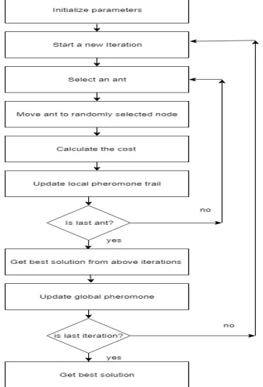
When ants move from point A (source) to point B (target), ants leave a chemical (pheromone) to mark these paths. This helps the following ants find the way their teammates find themselves when they detect pheromones and are more likely to choose paths with a higher concentration of pheromone. The algorithm is based on the adaptive adaptation of the pheromone on the routes at each node and is shown in Fig 1. The selection of this node is based on a probability-based selection approach.

The ants are driven according to a probability rule to choose their solution to the problem called the Tour. The probability rule between two nodes i, j, called the pseudo-random proportional action-choice rule, depends on two factors: the heuristic and the metaheuristic.

= ………. (2)

Where τ is the pheromone, η is the inverse of the distance between the two nodes. Each ant modifies the environment in two different ways:

1) Local trail updating: As the ant moves between nodes it updates the amount of pheromone on the edge by using an equation, which is given below:

(t) = (1-ρ). (t-1) + ρ. ……… (3)

Where, ρ is the evaporation constant. The value is the initial value of pheromone trails and can be calculated as:

= (n / )-1………. (4)

Where, n is the number of nodes and the total distance covered between the total nodes, produced by one of the construction heuristics.

2) Global trail updating: When all nodes have traversed by all the ants than it finds the shortest path updates the edges in its path using the following equation

(t) = (1-ρ). (t-1) + ……… (5)

Where, is the length of the best path generated by one of the ants.

B. Genetic Algorithm (GA)

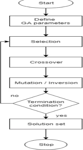
The genetic algorithm is started with a set of solutions (represented by chromosomes) called populations. Solutions from a population are taken and used to form a new population. This is motivated by the hope that the new population is better than the old one. Solutions chosen to form new solutions (descendants) are selected according to their suitability; The more appropriate they are, the more chances they have of reproducing themselves. This is repeated until a condition (e. g, number of populations or best solution improvement) is met. It is well known that problem solving can often be expressed as looking for the extreme of a function. This is exactly the case with the following problem: Some functions are given and GA tries to find the minimum of the function.

1) Start,

2) Generate random population of n chromosomes (Define parameters),

3) Evaluate the fitness f(x) of each chromosome x in the population (fitness),

4) Create a new population by repeating the following steps until the new population is complete,

a) Select two parent chromosomes from a population according to their fitness (the better fitness, the bigger chance to be selected that is Selection)

b) With a crossover probability cross over the parents to form a new offspring (children). If crossover was not performed, then offspring is a copy of parents (Crossover).

c) With a mutation probability mutate new offspring at each locus (position in chromosome that is Mutation)

d) Place new offspring in a new population (Accepting).

5) Use new generated population for a further run of algorithm (Replace),

6) If the end condition is satisfied, go to step 7 return the best solution in current population (check the condition), else go to step 4

7) Get solution set,

8) Stop

The above outline of GA is very general. There are many things that can be implemented differently in various problems. The basic steps of GA are explained in details as follows-

i) Representation: An initial population is created from a random selection of solutions (analogous to the chromosomes). It involves the representation of an individual (a possible solution or decision or hypothesis) in terms of its genetic structure (a data structure that represents a sequence of genes called chromosomes). At each point of the search process, a generation of people is maintained. The original population ideally has different individuals. This is necessary because individuals learn from each other. The lack of diversity of the population leads to suboptimal solutions. The initial diversity can be arranged by uniform random, grid initialization, non-clustering or local optimization methods [16].

ii) Evaluation: Each solution (chromosome) is assigned a value for fitness, depending on how close it actually is to solving the problem (and thus solving the desired problem). The fitness function is a measure of the goal to be achieved (maximum or minimum values). The fitness function is optimized using the genetic process and evaluates each solution to determine if it will contribute to the next generation of solutions. Since it selects which individuals can reproduce and create the next generation of the population, it is designed with care.

iii) Selection: The selection of individuals for the next generation to reproduce or to live strongly depends on the evaluation function. Those higher-fitness chromosomes are more likely to reproduce progeny (which can mutate after reproduction). The offspring is a product of the father and the mother whose composition consists of a combination of genes of them (this process is called "crossing over"). After judging the suitability of the individuals, the selection of the "suitable" individuals for reproduction / recombination is performed by applying the evaluation function. The selection procedures that can be used are deterministic selection, proportional fitness, tournament selection, etc. Each technique has its own advantages and disadvantages and can be selected according to the problem and the population.

iv) Recombination: Recombination or reproduction is like in biological systems, candidate solutions combine to produce descendants in every algorithmic iteration called generation. From the generation of parents and children, the strongest survive to become candidate solutions in the next generation. Offspring are produced by certain genetic operators such as mutation and recombination.

In recombination, one or more pairs of individuals are randomly selected as parents and segments (genes) of the parents are randomly exchanged. Solutions combine to create new generation for the next generation. Sometimes they pass on their worst information, but if recombination is done in combination with a powerful selection method, better solution results are achieved. Recombination can be performed using various methods such as 1-point recombination, N-point recombination, and uniform recombination.

Mutation is the most fundamental way to change a solution for the next generation. Operators of the local search techniques can be used to easily work with the solution and introduce new random information. It is thus affected by randomly changing one or more digits (genes) in the string (chromosomes) representing a person. In binary coding, this may simply mean changing a 1 to a 0 and vice versa [16].

C. The Hybrid of Genetic Algorithm with Ant Colony Optimization (GA-ACO)

There are several papers based on the hybridization of GA and ACO. Shang et. al. proposed to hybridize GA and ACO as a new algorithm for solving TSP [17]. GA is benefited in this work by initiating the pheromone matrix in ACO and recombining the route of ACO. The author claimed that the hybrid algorithm was more effective compared to GA and ACO. Duan and Yu suggested using a memetic algorithm to find the combination of parameters in ACO [18]. The author claimed that this hybridization would simplify the selection of the adjustable parameter in ACO when human experience is required and, in most cases, depends on chance. Jin-Rong et al. developed two GA and ACO hybridization-based sub algorithms that cover the weaknesses of both algorithms [19]. ACO is used to help GA eliminate the occurrence of an invalid trip, while GA is used to overcome dependence on the pheromone matrix in ACO. Al-Salami developed a hybrid of ACO and GA algorithm by combining each base method as a sub-solution generator and then they select the better sub-solution as a new population for the next iteration [20]. In this work, ACO is used as a temporary solution generator, which is improved by iterative implementation of GA operators until the stop criteria is reached. Takahashi proposed GA and ACO hybridization, which is slightly more efficient than Al-Salami's work by extending the GA (EXO) crossover operator to produce a better solution produced by ACO [21]. There are two steps to getting the solution. First, use ACO to generate the solution that has achieved the local optima. Solution creation in this step is repeated iteratively and independently. Such a solution is then treated as a population in GA or, in other words, the chromosome that is recombined in GA to obtain better global optima. In a similar way, Dong et. al. The previous hybridization work has been improved by introducing GA as a sub-process in each iteration in ACO [22]. This proposed work will increase the likelihood of changing the route leading to ACO. However, the above work did not assume that the cycle depended on the previous one to prevent premature convergence in ACO. In this article, GA's chromosomes are used to optimize the number of next towns visited by each ant to avoid dependency on the previous cycle. From these chromosomes, the variety of ant inspection can be obtained. The next section shows the details of the proposed work.

1) Hybridization Technique: In this paper a suitable approach is used to hybridize GA and ACO to find a TSP solution that will construct the concept that combines certain steps in GA and ACO to perform GA-ACO. Hybridization is also applied to some parameters and variables of GA or ACO that have the same characteristics in the calculation, i.e. the population size in GA and the number of ants in ACO, the number of generations in GA and the number of cycles in ACO and the chromosome in GA and taboo list in ACO. The technique proposed in this thesis introduces the evolutionary steps of GA into the calculation step of ACO as shown in Table 4.1. The modification is shown in the flowchart.

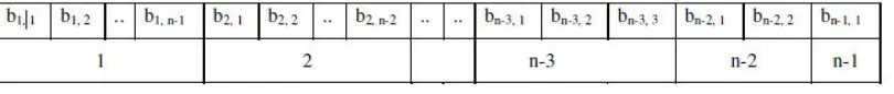
2) Chromosomal representation on GA-ACO: In the experiment, the performance of the proposed hybrid method is compared with the basic methods GA and ACO. In this case, a compatible chromosomal representation for GA and GACO must be appropriate. The binary representation is therefore chosen reasonably. These representations guarantee that solutions obtained by classic operators are valid. For these representations, no special operators need to be defined. To solve the TSP of n cities, the chromosome representation is structured as follows:

a) Each chromosome contains (n-1) groups of genes.

b) The number of genes in group i is equal to (n-i) bit, so that the total number of genes ( ) in the chromosome follows equation (4.7)

= ……….. (6)

Fig 3: Chromosomal Representation of n Cities

In basic GA, the chromosome represents the TSP solution indirectly. Here is the process to decode the chromosome to the TSP solution:

a) The indexes of cities not visited are defined as a set called allowed.

b) The city visited is determined by the number of genes 1 in the gene groups. If the number of gene 1 is k, then the city visited is the allowed kth index. If there is no gene 1 in the ith group, then the city visited is the last allowed index.

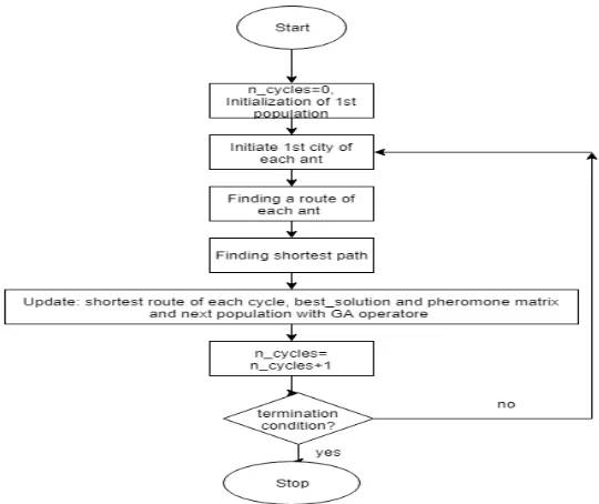
Fig 4: Flowchart of GA-ACO

1) Step 1: Start

2) Step 2: Set genetic algorithm parameters and ant colony parameters

3) Step 3: Generate initial random population

4) Step 4: Evaluate fitness for each chromosome in the population

5) Step 5: Start ACO

6) Step 6: Create ants

7) Step 7: Put ants on an entry state

8) Step 8: For each ant, create the empty path lists

9) Step 9: Select next state for each ant

10) Step 10: Update local pheromone

11) Step 11: Update global pheromone

12) Step 12: Evaporate pheromone

13) Step 13: End ACO

14) Step 14: Parents selection for next chromosome

15) Step 15: Crossover of parent’s chromosome

16) Step 16: New population

17) Step 17: Criteria met? If yes move to the next step, else go to step 4

18) Step 18: End

The number of bits 1 is used in the group of genes to determine the cities that the ants can visit. The determination process follows:

a) The indexes of cities not visited are defined as a set called allowed.

b) The first city visited is determined by the number of gene 1 in the first gene groups directly. If the number of gene 1 is c, then the first city visited has a cth rate allowed. If there is no gene 1 in the first group, then the first city visited is the last allowed index.

c) For the other cities, the number of genes 1 is used in another group of genes and equations (7) to determine the cities that will be visited one by one. If there is no gene 1 in the ith group of the gene, then equation (7) is used as the basic ACO, all allowed indices have the opportunity to be visited according to their probabilities. If there is only one gene 1, the city visited is the city that has the highest probability as a consequence. And if the number of gene 1 is c, then only the first c indices allowed have the opportunity to be visited. Equation (7) is a formula by Dorigo et al [17] to find the next city to visit.

where α and β are parameters that control the relative importance of the trajectory versus visibility, k is the index of ant, allowedk is the set of unvisited cities that will probably be visited by kth ant, i is the index of the last city currently visited, j is the index of the next city that visited the city, t is the time index, τ is the intensity of the trail and h is the visibility.

a) Once a city has been configured to be visited, the city's index is deleted as allowed.

b) The last index that is allowed is the last city visited.

III.EXPERIMENTALSETUP,RESULTSANDANALYSIS

The experimental results for each method are obtained by using the given evaluation parameters for simulation: -

1) For basic GA, the crossover probability Pc is 0.4, and mutation probability Pm is 0.6, and population is 100. In addition, the crossover method used is uniform random crossover. The number of iterations is changed like for first cycle it is 50 and then for second it is 100. For both the cycles the number of cities will be vary like 10, 20, 30, 40, 50 and 60.

2) For basic ACO, α is 1, β is 1, ρ is 0.4817, a constant of the trail quantity Q is 1, τ is blank initially and number of ants are 100. The number of iterations is changed like for first cycle it is 50 and then for second it is 100. For both the cycles the number of cities will be vary like 10, 20, 30, 40, 50 and 60.

3) For GA-ACO, Pc is 0.1, Pm is 0, α is 1, β is 2, ρ is 0.4817, τ is blank initially, and Q is 1, population is 100. In addition, the crossover method used is also uniform random crossover. The number of iterations is changed like for first cycle it is 50 and then for second it is 100. For both the cycles the number of cities will be vary like 10, 20, 30, 40, 50 and 60.

A. Parameters Used for Comparative Study of GA, ACO and GA-ACO

The various parameters which have been used for the comparative study of GA, ACO and GA-ACO are explained below: -

1) Cost: - In this simulation, the cost is the distance covered to traverse all the given cities exactly once. Various algorithms are used to find the cost in this simulation. It will find out all the possible paths but at the end the minimum cost will be reflected by that algorithm i. e. GA, ACO and GA-ACO.

2) Fitness Achieved: - In genetic algorithms, each solution is usually represented as a string of binary numbers, known as a chromosome. We have to test these solutions and find the best set of solutions to solve a given problem. Therefore, each solution must receive a score to indicate how close it was to meet the general specifications of the desired solution. This score is generated by applying the physical fitness function to the test, or the results obtained from the tested solution.

3) Time: - Here, in the simulation the time parameter stands for the time consumed to find all the possible paths by each algorithm. Here one will select the algorithm to find the optimal path, so that when the algorithm will start the time parameter will start working and reflects the total time consumed to find all the solution given by that algorithm. In short. The time taken to execute all the number of iterations is given by time parameter.

TABLE 1: RESULT OF SIMULATION OF ACO, GA, GA-ACO

Number of Cities Number Of Iterations Populati on

ACO GA GA-ACO

Initial Score

Final Score

Time Cost Initial Score

Final Score

Time Cost Initial Score

Final Score

Time Cost 10 50 100 0.17374 0.29316 35.4523 3.4111 0.27463 0.37019 38.4953 2.7013 0.17374 0.29383 10.2937 3.4033

20 50 100 0.084004 0.3085 35.4005 3.2415 0.13239 0.16865 37.0315 5.9295 0.08400 4

0.3085 13.8979 3.2415 30 50 100 0.06875 0.24646 37.5472 4.0575 0.088897 0.11184 37.4284 8.9416 0.06875 0.25432 19.1619 3.932 40 50 100 0.052173 0.1997 35.6031 5.0076 0.068191 0.07135 36.9172 14.015

5

0.05217 3

0.20354 18.5752 4.9131 50 50 100 0.0393386 0.16201 35.8643 6.1723 0.043918 0.01352 37.1812 19.473

3

0.03938 6

0.16451 21.989 6.0786 60 50 100 0.030237 0.14587 36.2981 6.8554 0.036278 0.040202 37.1216 24.874

1

0.03023 7

0.15341 26.9598 6.5185 10 100 100 0.24173 0.42489 69.711 2.3536 0.39322 0.53474 86.143 1.8701 0.24173 0.42489 15.584 2.3536 20 100 100 0.11615 0.24997 71.686 4.0005 0.12748 0.17949 73.7268 5.5714 0.11615 0.25566 30.7655 3.9114 30 100 100 0.062764 0.21878 70.1117 4.5707 0.08375 0.11351 74.0612 8.8095 0.06276

4

0.21883 33.1139 4.5697 40 100 100 0.045438 0.17936 72.9003 5.5754 0.056224 0.071313 73.0256 14.022

7

0.04543 8

0.1875 50.3449 5.3333 50 100 100 0.039453 0.15841 71.6334 6.3129 0.046392 0.059578 73.056 16.784

8

0.03945 3

0.16124 76.5717 6.202 60 100 100 0.031663 0.14656 80.003 6.8231 0.036553 0.042724 72.9754 23.406

3

0.03166 3

Fig 5: Comparison of Fitness Achieved at 50 Iterations

Fig 5 shows fitness achieved at 50 iterations for GA, ACO and GA-ACO at varying number of cities 10, 20, 30, 40, 50 and 60. It is clearly seen from the graph that GA-ACO and ACO gives almost same result. At first point i. e. at 10 cities GA gives good fitness but as number of cities increases its fitness getting down in exponential manner.

Fig 6: Comparison of Cost at 50 Iterations

Fig 6 shows cost achieved at 50 iterations for GA, ACO and GA-ACO at varying number of cities 10, 20, 30, 40, 50 and 60. It is clearly seen from the graph that GA-ACO and ACO gives almost same result but GA-ACO is giving slightly minimum cost. In GA as the number of cities increases the computational cost of the algorithm increases in exponential manner.

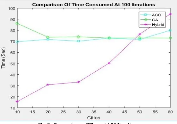
Fig 7 shows time consumed at 50 iterations for GA, ACO and GA-ACO at varying number of cities 10, 20, 30, 40, 50 and 60. It is clearly seen from the graph that GA consumed highest time to give all the possible paths, whereas ACO takes small time in compare to GA. But GA-ACO takes smallest time to give the all possible paths that can be traversed.

Fig 8: Comparison of Fitness Achieved At 100 Iterations

Fig 8 shows fitness achieved at 100 iterations for GA, ACO and GA-ACO at varying number of cities 10, 20, 30, 40, 50 and 60. It is clearly seen from the graph that GA-ACO and ACO gives almost same result. At first point i. e. at 10 cities GA gives good fitness but as number of cities increases it gives worst fitness, whereas the fitness achieved by ACO and GA-ACO are approximately same as the number of cities increases.

Fig 9: Comparison of Time at 100 Iterations

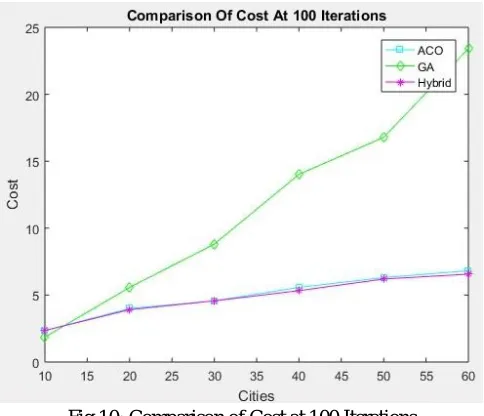
Fig 10: Comparison of Cost at 100 Iterations

Fig 10 shows cost achieved at 100 iterations for GA, ACO and GA-ACO at varying number of cities 10, 20, 30, 40, 50 and 60. It is clearly seen from the graph that GA-ACO and ACO gives almost same result. At 10 cities GA gives minimum cost but as number of cities increases its cost is increasing continuously quite higher. The cost factor is not increasing that high as the number of cities increases in ACO, GA-ACO

It is definitely an unexpected finding that in all the cases GA performs worst. GA-ACO gives better solution, with minimum time and cost. For example, we can compare the best solution for 30 cities and 50 iterations. In this case, the cost factor of GA-ACO 3.932 and the cost factor of ACO is 4.0575, whereas for GA cost factor is 8.9416, which is quite higher than the other two algorithms. When we conclude the result, it is observed that, in each case the result of hybrid GA-ACO is better than other two algorithms. The comparison shows that GA-ACO is better than other two but in case of fitness achieved ACO matches the values of GA-ACO sometimes. When the number of iterations is increased the performance of GA also improved and it shows better result with higher number of iterations.

IV.CONCLUSIONS

In this paper a study of optimization algorithms for TSP has been simulated through MATLAB and also proposed a hybrid optimization algorithm based on GA and ACO under various scenarios considering the different parameters for affecting the performance of optimization. All the algorithms are compared on the basis of three parameters that are Cost, Time and Fitness Achieved. In this work all the algorithms using three parameters are being simulated on two cases i. e 50 iterations and 100 iterations. The results obtained through simulations have been analyzed and evaluated for GA, ACO and proposed algorithm (GA-ACO), it is concluded as under: -

A. It is concluded that in large population the performance of ACO is better than GA whereas the performance of proposed algorithm i.e. GA-ACO is better than GA/ACO; which gives minimum cost in the GA-ACO compare to GA/ACO due to better heuristic value parameter of ACO.

B. The time consumed to execute GA-ACO is also lesser than GA and ACO algorithms due to the parallel search over several constructive computational threads using by ACO.

C. The fitness achieved by the GA-ACO is slightly improved than the GA and ACO algorithms because it is inversely proportional to cost factor i. e. if cost is minimum then the fitness achieved is higher.

V. ACKNOWLEDGMENT

I would like to express my deepest appreciation to all those who provided me the possibility to complete this paper. It would not have been possible without the kind support and help of many individuals and the institute. I would like to extend my sincere thanks to all of them. I am highly indebted to my supervisor Dr. N. C. Barwar for his guidance and constant supervision as well as for providing necessary information regarding writing this paper. His motivation has helped me pursue my work in the field of Optimization Techniques for Traveling Salesman Problem.

REFERENCES

[1] S. Koziel and X.-S. Yang, “Computational optimization, methods and algorithms” vol. 356. Springer, 2011. [2] M. Mitchell, An Introduction to genetic algorithms. MIT Press, 1998.

[3] J. Kennedy and R. Eberhart, “Particle swarm optimization,” Neural Networks, 1995. Proceedings., IEEE Int. Conf., vol. 4, pp. 1942–1948 vol.4, 1995. [4] M. Dorigo, M. Birattari, and T. Stutzle, “Ant colony optimization,” IEEE Comput. Intell. Mag., vol. 1, no. 4, pp. 28–39, 2006.

[5] A. Mucherino, O. Seref, O. Seref, O. E. Kundakcioglu, and P. Pardalos, “Monkey search: a novel metaheuristic search for global optimization,” in AIP conference proceedings, 2007, vol. 953, no. 1, pp. 162–173.

[6] C. Yang, X. Tu, and J. Chen, “Algorithm of marriage in honey bees optimization based on the wolf pack search,” Proc. 2007 Int. Conf. Intell. Pervasive Comput. IPC 2007, pp. 462–467, 2007.

[7] X.-S. Yang and S. Deb, “Cuckoo search via Lévy flights,” in Nature & Biologically Inspired Computing, 2009. NaBIC 2009. World Congress on, 2009, pp. 210–214.

[8] W. Pan, “Knowledge-Based Systems A new Fruit Fly Optimization Algorithm Taking the financial distress model as an example,” Knowledge-Based Syst., vol. 26, pp. 69–74, 2012.

[9] A. Kaveh and N. Farhoudi, “A new optimization method: Dolphin echolocation,” Adv. Eng. Softw., vol. 59, pp. 53–70, 2013. [10] S. Mirjalili and A. Lewis, “The Whale Optimization Algorithm,” Adv. Eng. Softw., vol. 95, pp. 51–67, 2016.

[11] X. Chen, Y. Kong, X. Fang, and Q. Wu, “A fast two-stage ACO algorithm for robotic path planning,” Neural Comput. Appl., vol. 22, no. 2, pp. 313–319, 2013. [12] Ivan Brezina Jr., ZuzanaCickova, “Solving the Travelling Salesman Problem using the Ant colony Optimization”, Management Information Systems, 2011,

Vol. (6), No. (4).

[13] ButhainahFahran, Al-Dulaimi, and Hamza A. Ali, “Enhanced Traveling Salesman Problem Solving by Genetic Algorithm Technique (TSPGA)”, World Academy of Science, Engineering and Technology, 2008, Vol. (14).

[14] Dorigo M, Stützle T. Ant Colony optimization. Cambridge, MA: MIT Press; 2004.

[15] Dorigo M, Maniezzo V, Colorni A. Ant System: Optimization by a colony of cooperating agents. IEEE Trans Syst Man Cybernet Part B 1996;26(1):29–41. [16] Prof. Swati V. Chande and Dr. Madhavi Sinha “Genetic Algorithm: A Versatile Optimization Tool” in BIJIT - BVICAM’s International Journal of Information

Technology Bharati Vidyapeeth’s Institute of Computer Applications and Management (BVICAM), New Delhi.

[17] Shang, G., Xinzi, J., Kezong, T., (2007), Hybrid Algorithm Combining Ant Colony Optimization Algorithm with Genetic Algorithm, in Proc. of the 26th Chinese Control Conf.

[18] Duan, H., Yu, X., (2007), Hybrid Ant Colony Optimization Using Memetic Algorithm for Traveling Salesman Problem, in Proc. IEEE Int. Symposium. Dynamic Programming and Reinforcement Learning.

[19] Jin-rong, X., Yun, L., Hai-tao, L., Pan, L., (2008), "Hybrid Genetic Ant Colony Algorithm for Traveling Salesman Problem", J. Computer Applications, Vol. 28, No. 8, pp2084-2112.

[20] Takahashi, R., (2009), A Hybrid Method of Genetic Algorithms and Ant Colony Optimization to Solve the Traveling Salesman Problem, in Proc. Int. Conf. Machine Learning and Applications.

[21] Al-Salami, N. M. A., (2009), "Ant Colony Optimization Algorithm", J. UbiCC, Vol. 4, No. 3, pp823-826.