Aboveground biomass estimation in linear forest objects: 2D- vs. 3D-data

JOURNAL OF FOREST SCIENCE, 64, 2018 (12): 523–532

https://doi.org/10.17221/106/2018-JFS

Aboveground biomass estimation

in linear forest objects: 2D- vs. 3D-data

Stefan LINGNER*, Eiko THIESSEN, Eberhard HARTUNG

Institute of Agricultural Engineering, University of Kiel, Kiel, Germany *Corresponding author: [email protected]

Abstract

Lingner S., Thiessen E., Hartung E. (2018): Aboveground biomass estimation in linear forest objects: 2D- vs. 3D-data. J. For. Sci., 64: 523–532.

Wood-chips of linear forest objects (hedge banks and roadside plantings) are used as sustainable energy supply in wood-chip heating systems. However, wood yield of linear forest objects is very heterogeneous and hard to estimate in advance. The aim of the present study was to compare the dry mass estimation potentials of two different non-destructive data: (i) Canopy area (derived from aerial images) and mean age at stump level (2D), (ii) volume of veg-etation cover based on structure from motion (SfM) via unmanned aerial vehicle (3D). These two types of data were separately used to predict reference dry mass (ground truth) in eleven objects (5 hedge banks and 6 roadside plant-ings) in Schleswig-Holstein, Germany. The predicting potentials were compared afterwards. The reference dry mass was ascertained by weighing after harvesting and drying samples to constant weight. The model predicting reference dry mass using canopy area and mean age at stump level achieved a relative root mean square error (RMSE) of 52% (42% at larger combined plot sizes). The model predicting reference dry mass using SfM volume achieved a relative RMSE of 30% (16% at larger combined plot sizes). This result indicates that biomass is better described by volume of vegetation cover than by canopy area and age.

Keywords: SfM; aerial images; hedge banks; roadside plantings; UAV; dry biomass

According to the European Renewable Energy Directive (2009/28/EG) renewable energy is sup-posed to cover at least 20% of the gross energy consumption in 2020 within the European Union. In Germany, the amount of woody biomass used as a source for energy has already increased during the last decades (Mantau 2012). The future de-mand for woody biomass could in part be supplied by existing linear forest objects (hedge banks and roadside plantings) (Isensee et al. 2000; Seidel et al. 2015).

The demand of wood-chips implies the need for woody biomass predicting models. Biomass pre-dicting models could help with logistical planning and economical estimations. Biomass predictions

based on allometric equations were already com-pared to biomass predictions based on Structure from Motion (SfM) in a previous study (Lingner et al. 2018). Dry mass predictions based on SfM turned out to be comparably accurate. However SfM is time consuming and technically demanding.

SfM is a remote sensing technique that constructs 3D point clouds from numerous overlapping pho-tos. The underlying algorithms use methods of computer vision and photogrammetry. These algo-rithms are looking for key points in individual pho-tos and are matching these points with associated key points in other photos. Thus, the camera posi-tion and its calibraposi-tion plus the locaposi-tion of the key points are estimated. Afterwards these key points

are converted into a 3D point cloud (Snavely et al. 2007; Turner et al. 2012). Analysing these point clouds enables e.g. the calculation of arbitrary ori-ented distances within these points or the overall included volume.

For tree parameter estimation SfM top-down ap-proaches of leafy trees (Dandois, Ellis 2010; Tao et al. 2011; Fritz et al. 2013; Zarco-Tejada et al. 2014; Díaz-Varela et al. 2015) and SfM side-on approaches of bald trees (Miller et al. 2015) have been applied. SfM at bald trees allows the re-construction of pure wood and thus supposingly achieves high accuracies. However by now pure wood reconstruction has only been applied suc-cessfully to single trees (Miller et al. 2015). SfM at leafy trees for height estimations or coarse vol-ume models is less accurate but can be applied to grouped trees as well (Dandois, Ellis 2010; Fritz et al. 2013; Zarco-Tejada et al. 2014).

Predicting models based on aerial images instead of SfM volume models would be faster process-able and consequently more economical. Seidel et al. (2015) has used canopy area and age to pre-dict dry mass in linear forest objects in Germany. In this study the canopy areas were derived from aerial images. The growth rate was assumed to be 0.7 kg·m–2_·yr–1_.

The aim of the present study was to compare the predicting potential of these two different non-de-structive approaches. The first approach used can-opy area and mean age at stump level as predicting variables and the second approach used volume of vegetation cover based on SfM as predicting vari-able. The data of both approaches were used sepa-rately to predict reference dry mass (ground truth). Afterwards the predicting potentials of both ap-proaches were compared.

MATERIAL AND METHODS

Study objects. Data for the present study were sampled in 2016, 2017 and 2018 at eleven linear forest objects in Schleswig-Holstein, Germany. Average yearly temperature in Schleswig-Holstein is around 10°C and annual precipitation is around 750 mm. All objects were in an altitude of approxi-mately 30 m a.s.l.

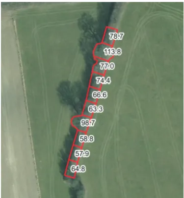
These objects consisted of five different hedge banks (objects 1 to 5) and six roadside plantings (ob-jects 6 to 11). A representative length of 100 m was selected for each object. The 100 m objects were di-vided into 10 segments of 10 m each. A Real Time Kinematic GPS (Trimble Ag 442 with 2 cm

horizon-tal accuracy) recorded the GPS coordinates of the segments’ corners.

Sampled hedge banks and roadside plantings had diverse species compositions. Some of the hedge banks had a large proportion of blackthorn (Prunus spinosa Linnaeus) other objects were dominated by willow (genus Salix Linnaeus), sycamore (Acer pseudoplatanus Linnaeus) or common hornbeam (Carpinus betulus Linnaeus). Most frequent count-ed shoots of all segments were blackthorn, fly hon-eysuckle (Lonicera xylosteum Linnaeus) and com-mon hazel (Corylus avellane Linnaeus).

Reference data. In the beginning of 2017 (Ob-jects 1, 2, 6, 7, 8) and 2018 (Ob(Ob-jects 3, 4, 5, 9, 10, 11) shrubs and trees of each segment were felled, chopped to wood-chips and weighed segment-wise. The vegetation was without leaves at that time. Due to local conditions the segments had to be weighted on four different scales (Table 1).

From each segment three samples of wood-chips (approximately 5 l each) were taken. These samples were dried at 103°C to constant weight according to DIN 52183 for dry mass content estimation. Thus the dry mass of every segment could be estimated.

Usually not all trees are felled in hedge banks and roadside plantings. Some trees are left standing for ecological reasons. However these trees were part of the SfM-volume models and aerial images. Con-sequently the dry masses of the trees left standing were estimated with species-specific allometric equations based on DBH provided by Zianis et al. (2005). These dry masses were added to the har-vested dry masses to gain the total reference dry masses per segment.

Biomass estimation based on canopy area and age. The following prediction model is based on the idea that age could potentially be a substitute for tree height and that the canopy area could potentially be a substitute for basal area. Basal area in forest ecolo-gy is the sum of the area of all stems at breast height. Canopy area in the present study is the area covered by the combined canopy of the segment.

Consequently the Eq. 1.2 approximates the Eq. 1.1: Dry mass a tree height basal area _(1.1) Dry mass b age canopy area _(1.2)

(Version 2.18.22, 2017). The ages of the objects were estimated after harvesting by annual ring counting of 20 representative stumps per object. The mean age per object was used as object age. This mean rep-resents the period since the last harvest and there-fore the time duration for biomass growth used in Eq. 1.2. Seidel et al. (2015) recommended to esti-mate dry mass of linear forest objects based on can-opy area and age using Eq. 1.2 with 0.7 kg·m–2_·yr–1 _as

prefactor b.

Two models were generated. In Model 1.2a, 0.7 kg·m–2_·yr–1 _{was used as b in Eq. 1.2. For Model}

1.2b the prefactor b was estimated anew using the 110 data points of the present study.

Biomass estimation based on SfM volume of vegetation cover. For image acquisition an

un-manned aerial vehicle – UAV (HT-8 C180; Height-Tech, Germany) equipped with a Sony Alpha 7 camera (Sony Corporation, Japan), 24 mega pixel, 30 mm lens (Zeiss, Germany) was used. This cam-era and lens combination resulted in a pixel size of 6 mm × 6 mm at a distance of 30 m. The octocop-ter was programmed and flew automatically above and along each object in multiple different heights (Lingner et al. 2018). At the hedge banks the octo-copter could fly above the object and on both sides. However at the roadside plantings the octocopter could only fly on the opposite side of the road and above the object due to safety reasons.

The UAV flights were performed in the second half of 2016 (Objects 1, 2, 6, 7, 8) and in the second half of 2017 (Objects 3, 4, 5, 9, 10, 11) with most of the trees still leafy.

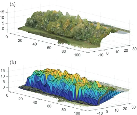
Approximately every two metres a photo was taken. This resulted in an overlap of more than 90% between collected images. Images were processed in Agisoft Photoscan (Version 1.2.6, 2016) for point cloud generation (alignment: highest; dense cloud: lowest). Then these point clouds were processed in Matlab (Version R2017a). The point cloud process-ing in Matlab included ground level estimation and volume calculation. For volume calculation square tiles with a uniform tile edge length (see below) were fitted at the estimated ground level. These tiles were used as base for pillars that reached from the estimated ground level to the highest point above the specific tile (Fig. 2). Square tiles with different edge lengths were tested on a sub sample to find the best suitable tile edge length. Tested tile edge lengths were d/n (n = 1…15) to fit exactly into the segments with a length of d = 10 m.

Table 1. Different scales used for weighing

Hedge banks Roadside plantings

2017

scale No. 1 2

object 1–2 6–8

scale telescopic handler permanent truck scales

minimum load used (t) 0.7 6.9*

maximum load used (t) 1.2 27.7*

resolution (kg) 50 20

maximum possible load (t) 5 50

2018

scale No. 3 4

object 3–5 9–11

scale mobile truck scales permanent truck scales

minimum load used (t) 1.1* 6.5*

maximum load used (t) 2.2* 25.7*

resolution (kg) 10 20

maximum possible load (t) 20 50

*weights include tare

Two different models were generated for biomass estimation based on volume. In Model 2.1, the vol-umes of the pillars V_i were simply added segment wise yielding the total volume SV_j = ΣV_i of seg-ment j. These segment volumes SV_j were modelled against reference dry mass_j (kg) in Eq. 2.1 to esti-mate the coefficient c. Model 2.1 was generated for every tested tile edge length to find the best fitting tile edge length based on relative root mean square error (rRMSE). This best fitting tile edge length was used for further analysis (Model 2.1 and 2.2): Dry massj  c SVj (2.1)

For Model 2.2, Eq. 2.2 was fitted to obtain estimates for factor d and exponent f. This equation allows for different volume specific densities depending on pillar height. This could possibly rather represent the natural growth habit of trees then Eq. 2.1. Due to the fact that higher trees usually have a thicker stem than smaller trees, a higher pillar probably has a higher wood-air-ratio than a smaller pillar:

 

Number in 1

Dry mass_j d



where:

V_i – pillar volume (m3_),

j – segment number.

Different plot sizes. When the trees were weighed segment-wise (10 m) it was often hard to decide to which segment a tree belonged. Especially at the edges of the segments it was challenging to assign all trees to a distinct segment. Plus, if the crown of a tree covered parts of two adjacent segments the tree was not split apart. These edge errors resulted

by assigning trees to the wrong segment probably resulted in wrong reference data. It was tried to de-crease these edge errors test-wise by using larger plot sizes for both Model 1.2b (canopy area & age) and Model 2.1 (volume). Compared additional plot lengths were 20, 50, and 100 m when combining 2, 5, or 10 adjacent segments respectively.

To evaluate the accuracy of both biomass esti-mation approaches for applications in the field the 95% confidence intervals of the standard deviation (CI_SD) were calculated. These two CI_SD were cal-culated using the residuals of Model 1.2b and 2.1. Afterwards each CI_SD was converted into a relative CI_SD by dividing it by the mean reference dry bio-mass. For this calculation the plots with a length of 100 m were used since these plot sizes are more common at applications in the field.

Data handling, statistics and graphics. The ab-solute root mean square error (RMSE) or rRMSE is the standard accuracy estimate for the compari-son of different methods of biomass estimation (Segura et al. 2006; Hyde et al. 2007; Popescu et al. 2011). Consequently this accuracy estimate was used in the present study as well. The formula for the rRMSE (%) is presented in Eq. 3:





1

1

rR SE M ˆ n

i i i y y n

y

 





where:

y– – mean value, yˆ – expected value.

Data handling, statistics and graphics were per-formed in R software (Version 3.2.1, 2015) using the packages xlsx (Version 0.5.7, 2014), plyr (Ver-sion 1.8.4, 2011), mgcv (Ver(Ver-sion 1.8-24, 2018) (Wood 2011) and ggplot2 (Version 2.1.0, 2009) (Wickham 2009).

RESULTS

Reference data

Fresh biomass per segment varied between 380 and 8,380 kg and dry biomass content varied be-tween 47 and 66%. This resulted in harvested dry biomasses between 237 and 4,649 kg per 10 m seg-ment (Fig. 3a). In total, 66 trees with a DBH larger than 10 cm were left standing. Their dry masses were estimated with equations from Zianis et al. (2005) and added to the harvested dry biomasses to gain reference dry biomasses (Fig. 3b). These reference dry biomasses varied between 243 and

Fig. 2. Coloured point cloud of roadside planting (700,000 points) (a), point cloud with estimated ground level and pillars (2 m × 2 m at ground level) for volume calculation (b) (distances in metres)

(a)

4,800 kg per segment (10 m). The mean estimated dry mass of the trees left standing per segment was around 9% of the reference dry mass.

Biomass estimation based on canopy area and age

Digitizes canopy areas per segment varied be-tween 30 and 258 m2_{. The mean age of the objects}

ranged from 13 to 32 years. Ages and canopy ar-eas are displayed in Fig. 4. Estimated prefactor b in Model 1.2b was 0.44 kg·m–2_·yr–1_.

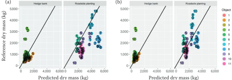
Fig. 5 shows both the estimated dry biomass with a prefactor b of 0.7 kg·m–2_·yr–1 _{(Model 1.2a)}

and the estimated dry biomass with the calculated prefactor b of 0.44 kg·m–2_·yr–1 _{(Model 1.2b). Model}

1.2a resulted in an rRMSE of 82% and Model 1.2b resulted in an rRMSE of 52%. An overview of the models is presented in Table 2.

Fig. 3. Harvested dry biomass (a), reference dry biomass – harvested dry biomass plus estimated dry biomass of trees left standing (b) of eleven linear forest objects

H

ar

ve

st

ed dr

y bioma

ss (kg)

Object Object

Ref

er

enc

e dr

y bioma

ss (kg)

(a) (b)

Fig. 4. Canopy area of segments – digitized in aerial images (a), age of objects – ascertained by annual ring counting (b); the points represent means and the error bars represent standard errors, sample size = 20 for each object

Object Object

Ar

ea (m

2)

Ann

ual r

ing

s (y

r)

(a) (b)

Fig. 5. Predicted dry biomass (Eq. 1.2) with two different growth factors vs. reference dry biomass: 0.7 kg·m–2_·yr–1 _(a), 0.44 kg·m–2_·yr–1 _{(b); the 1:1 line is also displayed and represents an ideal fit}

Ref

er

enc

e dr

y ma

ss (kg)

(a) (b)

Biomass estimation based on SfM volume

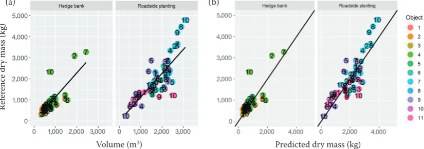
The best fitting tile edge length was found around 2 m. Edge lengths smaller or larger than 2 m resulted in a larger rRMSE. When using this tile edge length for further analysis the calculated volumes per 10 m segment varied between 286 and 3,088 m3 _{(Fig. 6). The}

estimate c in Eq. 2.1(Model 2.1) was 1.14 kg·m–3_{. The}

estimates d and f in Eq. 2.2(Model 2.2) were 0.28 and 1.38 respectively. Model 2.1 resulted in an rRMSE of 31% and Model 2.2 resulted in an rRMSE of 30%. The data points of both models are presented in Fig. 7. An overview of the models is presented in Table 2.

Different plot sizes

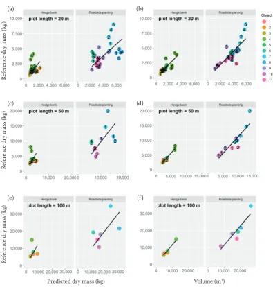
Data points of the larger plot sizes are presented in Fig. 8. The rRMSE values of the three additional plot lengths of the area and age model were 47% at 20 m, 43% at 50 m and 42% at 100 m. The rRMSE values of the three additional plot lengths of the SfM model were 27% at 20 m, 19% at 50 m and 16% at 100 m. At the 100 m plot sizes the residuals of Model 1.2b resulted in a relative 95% CI_SD of 82% and the residuals of Model 2.1 resulted in a relative 95% CI_SD 33%.

DISCUSSION

Data acquisition

Linear forest objects sampled were different in width, orientation, age and species composition to cover the broad scope of linear forest objects in Schleswig-Holstein. The ages of the objects (13 to 32 years) cover the broad scope of ages at which linear forest objects are harvested in Schleswig-Holstein (Ministerium für Energiewende, Land-wirtschaft, Umwelt und ländliche Räume des Landes Schleswig-Holstein 2017). The species compositions as well were a good representation of

Table 2. Models with equations, parameters, relative root mean square error (rRMSE) and 95% confidence intervals of the standard deviation (CI_SD) values

Model Equation rRMSE (%) CI_SD at 100 m (%)

1.2a _{Dry mass 0.70 kg·m ·yr} –2 –1_{age canopy area}

82 1.2b _{Dry mass 0.44 kg·m ·yr} –2 –1_{age canopy area}

52 82

2.1 Dry massj1.14 kg·m–3SVj 31 33

2.2 Dry mass 0.28 Number in 1

 

V j

j



dry mass in kg, j – segment number, SV_j – total volume, V_i – pillar volume (m3₎

Fig. 6. Volume calculations based on structure from motion of eleven linear forest objects

Fig. 7. Volume vs. reference dry biomass (Eq. 2.1 with a slope of c = 1.14), the line presents the linear model (a), predicted dry biomass vs. reference dry biomass (Eq. 2.2), the 1:1 line is displayed and represents an ideal fit (b)

Volume (m

3)

Object

Ref

er

enc

e dr

y ma

ss (kg)

Volume (m3_{) Predicted dry mass (kg)}

linear forest objects in Schleswig-Holstein (Eigner 1982). As a consequence the results of this study are likely to be applicable to all linear forest objects in Schleswig-Holstein. However the results might be less applicable to linear forest objects outside of Schleswig-Holstein.

Predicting potential

Accuracy of canopy area and age as predicting variables. Dry biomass estimation based on aerial images resulted in an rRMSE of 82% (Model 1.2a) and 52% (Model 1.2b). The spread of the data is the same in both models but the data points in Model 1.2a are further away from an ideal fit presented by a relation of 1:1. This difference explains the sub-stantially different rRMSE values.

Model 1.2a and Model 1.2b are predicting al-most the same dry biomass for every segment in a particular object (see the horizontal accumulation of points in Fig. 5). This pattern can in part be ex-plained by the fact that for all segments in a par-ticular object the same age was assumed. This as-sumption is rationally since usually an entire object is felled at one time. Consequently, all segments of an object have the same age when regrowing.

At larger plot sizes this method resulted in an rRMSE of 42%. The rRMSE values in literature for biomass estimation based on aerial images varied between 8% (Muukkonen, Heiskanen 2007), 14% (Ploton et al. 2012) and 40% (Muukkonen, Heis-kanen 2005). However reference data in these stud-ies were not gained by weighing but by less accurate techniques like allometric equations. So the rRMSE of these literature studies is not directly comparable

Fig. 8. Predicted dry masses (a, c, e), volumes (b, d, f) vs. reference dry masses at different plot sizes – 20 m (a, b), 50 m (c, d), 100 m (e, f) – gained by combining several adjacent plots

Canopy area and age Structure from motion volume

Ref

er

enc

e dr

y ma

ss (kg)

Ref

er

enc

e dr

y ma

ss (kg)

Ref

er

enc

e dr

y ma

ss (kg)

Predicted dry mass (kg) Volume (m3₎

(a) (b)

(c) (d)

to the present study since it is likely that a data set with a non-accurate reference method is worse than a data set with weighted reference values.

The present study could not confirm a growth rate of 0.7 kg·m–2_·yr–1 _{as recommended by Seidel et al.}

(2015). The calculated prefactor of 0.44 kg·m–2_·yr–1

in the present study was a lot smaller. Seidel et al (2015) guessed this prefactor for central Germany. The present study took place in northern Germa-ny. Walther and Bernath (2009) recommend a growth rate of 0.5 kg·m–2_·yr–1 _{for Switzerland. It is}

likely that this prefactor is different depending on climate, nutrition, species composition etc.

Accuracy of volume as predicting variable. Dry biomass estimation based on SfM-volume resulted in an rRMSE of 30% (Model 2.2). At larger plot sizes this method resulted in an rRMSE of 16%. This rRMSE is in the range of the rRMSE from Miller et al. (2015) who have used SfM to calculate the volume of thirty bald single trees and received an rRMSE of 19%. In Miller’s study the single trees were photographed side-on all around. Dandois and Ellis (2010) have used SfM for biomass estimation at a small forest and received an rRMSE of 54%. However, due to the large spatial scale they have used top-down photos only. Reference values were gained by allometric equa-tions. Consequently the rRMSE values should be compared with caution here as well.

The coefficient c was estimated to be 1.14 kg·m–3_.

Mean dry weight of the wood in hedge banks and roadside plantings in northern Germany is around 500 kg·m–3 _{(Verscheure 1998). Consequently the}

wood-ratio in a cubic metre of volume of vegeta-tion cover was at 0.2%.

The rRMSE of Model 2.2 was not much lower than the rRMSE of Model 2.1. The additional parameter for volume height did not improve the model no-tably. However the exponent was estimated to be larger than 1. Consequently higher pillars appear to have a higher wood-air-ratio than smaller pillars.

Comparison of accuracies. In the present study the rRMSE of the SfM-volume approach was small-er than the rRMSE of the approach based on asmall-erial images. It is not surprising that biomass is better described by volume than by canopy area since the canopy area in the optical images has no informa-tion about height. To substitute the height infor-mation age was added to the canopy area model (Model 1.2a and 1.2b). However, the canopy area model was still worse than the volume model. Ap-parently, age is no equal substitution for height at the scale of the present study.

Error analysis. The error of prediction is a com-bination of:

(i) the error of the reference dry biomass;

(ii) the error of the measurements (area and age or volume);

(iii) the heterogenetic allocation of dry mass in linear forest objects.

Reference dry biomasses were gained by weigh-ing after harvestweigh-ing. This is the most accurate method possible. Allometric equations based on DBH were used to predict the dry biomass of trees left standing. However, allometric equations from Zianis et al. (2005) are mainly from forest habitats. Consequently this dry biomass might be estimated inaccurate, since trees in a linear forest object have more light available and consequently are able to produce more biomass.

It was decided to stick to the equations from Zia-nis et al. (2005) for the following reasons:

(i) A tree that produces more biomass is likely to have a thicker stem as well. The equations used based on DBH. As a consequence the additional biomass would be taken into account;

(ii) Species-specific allometric equations for Euro-pean linear forest objects are rare in literature. Most equations are for forests or single trees. The width of the linear forest objects in the present study ranged from 7 m (hedge bank) to 22 m (roadside planting). The conditions in the centre of the objects are closer to a forest than to a single tree. Consequently equations for single trees would be less suitable.

Still, segments with estimated dry masses of trees left standing show a comparably bad fit in in Figs 5 and 7. The segments with the largest estimated dry masses were Segment 2, 7 and 10 of Object 4. The dry masses of these trees appear to be estimated too high.

Errors in area, age and volume estimation are assumed to be comparably small. Independent volume models were generated in different condi-tions and seasons for another project (unpublished data). It was shown that the calculated volumes had a high grade of reproducibility.

The allocation of dry mass was very heteroge-netic in the sampled linear forest objects. Some segments had a very dense vegetation, others seg-ments had large gaps in the centre. Some segseg-ments had a large part of small shrubs while others mainly consisted of a few large trees.

Different plot sizes. The rRMSE decreased con-siderably with increasing plot sizes. This effect is probably in part due to decreased edge errors. How-ever another reason surly is that errors are averaged in larger plot sizes and consequently disguised.

Applicability

In the present study the age of the objects was ascertained by annual ring counting after harvest-ing. Drill cores gained by growth ring drills could deliver this information semi-destructive. For an absolute non-invasive method this needs to be done in a different way (e.g. exploration of historic data).

Model 1.2b resulted in a relative 95% CI_SD of 82%. At a dry biomass of 10 t from typical 100 m hedge bank this CI_SD would result in a range between 2 and 18 t. Model 2.1 resulted in a relative 95% CI_SD of 33%. At a dry biomass of 10 t this CI_SD would result in a range between 7 and 13 t. The error of the models using aerial images is twice that high compared to the error of the volume models. Con-sequently, volume models should be preferred over models using optical images if smaller errors are essential.

References

Dandois J.P., Ellis E.C. (2010): Remote sensing of vegeta-tion structure using computer vision. Remote Sensing, 2: 1157–1176.

Díaz-Varela R., de la Rosa R., León L., Zarco-Tejada P. (2015): High-resolution airborne UAV imagery to assess olive tree crown parameters using 3D photo reconstruction: Appli-cation in breeding trials. Remote Sensing, 7: 4213–4232. Eigner J. (1982): Bewertung von Knicks in Schleswig-Holstein.

Laufener Seminarbeiträge No. 5/1982: 110–117.

Fritz A., Kattenborn T., Koch B. (2013): UAV-based pho-togrammetric point clouds – tree stem mapping in open stands in comparison to terrestrial laser scanner point clouds. The International Archives of the Photogrammetry, Remote Sensing and Spatial Information Sciences, XL-1/ W2: 141–146.

Hyde P., Nelson R., Kimes D., Levine E. (2007): Exploring LiDAR-RaDAR synergy – predicting aboveground biomass in a southwestern ponderosa pine forest using LiDAR, SAR and InSAR. Remote Sensing of Environment, 106: 28–38. Isensee E., Stübig D.K., Lubkowitz C. (2000): Bergung und

Aufbereitung von Knick- und Schwachholz. Landtechnik – Agricultural Engineering, 55: 346–347.

Lingner S., Thiessen E., Müller K., Hartung E. (2018): Dry Biomass Estimation of Hedge Banks: Allometric Equation

vs. Structure from Motion via Unmanned Aerial Vehicle. Journal of Forest Science, 64: 149–156.

Mantau U. (2012): Holzrohstoffbilanz Deutschland, Ent-wicklungen und Szenarien des Holzaufkommens und der Holzverwendung 1987 bis 2015. Hamburg, Universität Hamburg: 65.

Miller J., Morgenroth J., Gomez C. (2015): 3D modelling of individual trees using a handheld camera: Accuracy of height, diameter and volume estimates. Urban Forestry & Urban Greening, 14: 932–940.

Ministerium für Energiewende, Landwirtschaft, Umwelt und ländliche Räume des Landes Schleswig-Holstein (2017): January 20: Durchführungsbestimmungen zum Knickschutz. Kiel, Ministerium für Energiewende, Land-wirtschaft, Umwelt und ländliche Räume des Landes Schleswig-Holstein: 19.

Muukkonen P., Heiskanen J. (2005): Estimating biomass for boreal forests using ASTER satellite data combined with standwise forest inventory data. Remote Sensing of Envi-ronment, 99: 434–447.

Muukkonen P., Heiskanen J. (2007): Biomass estimation over a large area based on standwise forest inventory data and ASTER and MODIS satellite data: A possibility to verify carbon inventories. Remote Sensing of Environment, 107: 617–624.

Ploton P., Pélissier R., Proisy C., Flavenot T., Barbier N., Rai S.N., Couteron P. (2012): Assessing aboveground tropical forest biomass using Google Earth canopy images. Ecologi-cal Applications, 22: 993–1003.

Popescu S.C., Zhao K., Neuenschwander A., Lin C. (2011): Satellite lidar vs. small footprint airborne lidar: Comparing the accuracy of aboveground biomass estimates and for-est structure metrics at footprint level. Remote Sensing of Environment, 115: 2786–2797.

Segura M., Kanninen M., Suárez D. (2006): Allometric models for estimating aboveground biomass of shade trees and coffee bushes grown together. Agroforestry Systems, 68: 143–150.

Seidel D., Busch G., Krause B., Bade C., Fessel C., Kleinn C. (2015): Quantification of biomass production potentials from trees outside forests – a case study from Central Germany. BioEnergy Research, 8: 1344–1351.

Snavely N., Seitz S.M., Szeliski R. (2007): Modeling the world from internet photo collections. International Journal of Computer Vision, 80: 189–210.

Tao W., Lei Y., Mooney P. (2011): Dense point cloud ex-traction from UAV captured images in forest area. In: Proceedings of the 2011 IEEE International Conference on Spatial Data Mining and Geographical Knowledge Services (ICSDM 2011), Fuzhou, June 29–July 1, 2011: 389–392.

on Structure from Motion (SfM) point clouds. Remote Sensing, 4: 1392–1410.

Verscheure P. (1998) Energiegehalt von Hackschnitzeln – Überblick und Anleitung zur Bestimmung. Versuchs-bericht 1998/14. Freiburg im Breisgau, Forstliche Versuchs- und Forschungsanstalt Baden-Württemberg, Abteilung Arbeitswirtschaft und Forstbenutzung: 13.

Walther R., Bernath K. (2009): Energieholzpotenziale ausser-halb des Waldes. Studie im Auftrag des Bundesamtes für Umwelt (BAFU) und des Bundesamtes für Energie (BFE). Luzern, Interface Institut für Politikstudien, Zollikon, Ernst Basler + Partner AG: 82.

Wickham H. (2009): ggplot2: Elegant Graphics for Data Analysis. New York, Springer-Verlag: 213.

Wood S.N. (2011): Fast stable restricted maximum likelihood and marginal likelihood estimation of semiparametric generalized linear models. Journal of the Royal Statistical Society. Series B (Statistical Methodology), 73: 3–36. Zarco-Tejada P.J., Diaz-Varela R., Angileri V., Loudjani P.

(2014): Tree height quantification using very high resolu-tion imagery acquired from an unmanned aerial vehicle (UAV) and automatic 3D photo-reconstruction methods. European Journal of Agronomy, 55: 89–99.

Zianis D., Muukkonen P., Mäkipää R., Mencuccini M. (2005): Biomass and Stem Volume Equations for Tree Species in Europe. Helsinki, Finnish Society of Forest Science, Finnish Forest Research Institute: 63.