Function and evolution of genes in the human protein interaction network

Function and evolution of genes in the

human protein interaction network

by

˚

Asa P´erez-Bercoff

A thesis submitted to

The University of Dublin

for the degree of

Doctor of Philosophy

Department of Genetics

Trinity College

University of Dublin

This thesis has not been submitted as an exercise for a degree at any other University. Except where otherwise stated, the work described herein has

been carried out by the author alone. This thesis may be borrowed or

copied upon request with the permission of the Librarian, University of Dublin, Trinity College. This thesis may be deposited in the University’s open access institutional repository, subject to Irish Copyright Legislation and Trinity College Library conditions of use and acknowledgement. The

copyright belongs jointly to the University of Dublin and ˚Asa P´erez-Bercoff.

Signature of Author . . . . ˚

Asa P´erez-Bercoff

Acknowledgements

There are many to thank in this thesis. Obviously I will start with my supervisor Aoife McLysaght for unless she had let me join her group I would not be where I am today. So thank you for letting me join your group in my endeavour to understand molecular evolution and for supervision, and also for giving me the freedom to explore biological networks even when it meant collaborating and visiting the laboratory of another researcher. Therefore also my gratitude to collaborator Gavin Conant for letting me work together with you on such interesting topics, and also for letting me visiting your laboratory at the University of Missouri. Naturally I also wish to thank the past and present lab members in Aoife’s group: David, Kirsten, Takashi,

Dan, Fergal, Daniele and Aideen, and lab members in Gavin’s group: Micha¨el

and Corey. Also to Karsten at the Genetics department at TCD for being so helpful with computational matters, and even updating your paralogon data so that I could use it for the research in chapter 4. I enjoyed the company from all of you both in a scientific and a social capacity. I am grateful to have known and worked with all of you!

I also wish to thank participants of the Wednesday Lunch-time seminars at the Genetics department at TCD for interesting lectures and discussions, and at the University of Missouri, Chris Pires and members from his laboratory who joined Gavin Conant’s group for interesting scientific talks and discussions at the Wednesday network meetings.

paramount for my PhD! Thanks to my bosses Bernhard, Antonio, Andrea and Thierry at Adamans Ltd. for allowing me take some time off work so I could attend meetings with my supervisor once a month while I was working

for you. I am immensely grateful to G˚al¨ostiftelsen f¨or h¨ogre utlandsstudier

for giving me a very generous scholarship. With the money I received from you I not only paid the university fees of my final year, but my whole financial situation was sorted for the entire year. With this peace of mind as I did not have to worry about supporting myself anymore with a full-time job, and could therefore whole-heartedly focus on my research.

Thanks are also due to my former project supervisors Jens, Bengt and Lasse at Stockholm Bioinformatics Centre for supporting and encouraging me when I went to Ireland to undertake my PhD.

On a social note I would like to thank my friends. I have met many friendly and nice people while in Dublin, and in particular I wish to thank: my good house mates and friends Lilian (you are an incredible generous person, so thank you for so very much!) and Naisha (the three of us shared

much laughter in and out of the house!). Yonas (for alwayshearing me out, no

v

been mentioned above. A very special thank you to Joe and Shirley who after meeting my parents only once while diving in Spain housed me for free for two weeks upon my arrival in Dublin until I had my housing situation sorted. A thanks to Lilian’s aunt Janice and Lilian’s cousin Serena for letting me stay at your house when I have needed a place to stay, and to Naisha’s boyfriend Andrew for driving some of my belongings when I moved to my flat in Rathmines. Thanks to Kirsten’s (then boyfriend, now husband) Dan for together with Kirsten you two offered me a place to stay if I needed it. Thanks also to fellow cyclists Tim from the Genetics department who took me to Dublin 3DTri triahtlon club, and Nicholas captain of the TCD cycling club for cycling with and waiting for me so that I would not get lost around Meath, Kildare or up in the beautiful Wicklow mountains!

Thanks also to the people I got to know in Columbia Missouri that were so friendly to me. Especially my landlords Corey, Katy and your precious and sweet daughter Lulu (the memory of you still makes me smile), and also your friendly and protective dog Maggie. You all made me feel very welcome at your home, while I lived there during my time in Missouri. Thanks for inviting me to Sunday family dinners and other social events with your close friends. I am also glad to have met friends Ana, Armelle (thanks for offering to take me to see a doctor when I was home ill over Thanksgiving) and Damien from the French conversation group, and also Michela, and my Swedish next-door neighbour Rigmor and her husband Ronnie for their hospitality while I was in Missouri.

Thanks to friends I already knew back in Sweden (although not all of your are still there); Gabriel (thanks for bringing my racer bike over to Ireland for me!), Muna, Gabi and Kirsten; I am so glad you managed to visit me in Dublin. Thanks also to other friends I knew already before moving from Sweden especially Emelie, Marija and Nikola (I am honoured to have been

Abstract

The research conducted for this thesis aims to elucidate how the human protein interaction network has evolved, and how protein interactions

influence the spatial organisation of the metabolic network. The thesis

presents compelling results suggesting that indirect protein-protein inter-actions between metabolic enzyme proteins, and non-metabolic proteins

is a feature conserved from prokaryotes through to mammals. Indirect

protein-protein interactions are shown to influence the structure of metabolic networks, very likely through a mechanism called metabolic channelling. This mechanism brings metabolic pathway enzymes into close proximity of each other so that reactions between the enzymes can occur.

In E. coli and yeast, reactions that are linked to each other through mediator proteins have a much higher flux compared to reactions lacking them. The thesis presents indirect evidence that indirect protein-protein interactions are very important for the spatial organisation of metabolic protein networks. This thesis has also inferred the likely time of origin of the human protein-protein interactions that were examined, and suggests that most of the protein interactions in human are likely to be conserved in chimpanzee, macaque, mouse, rat, horse, dog and cow. This suggests they date from at least the point in evolution when placental mammals radiated out. Analyses of the function of proteins analyses in the thesis also suggests that the protein interactions have been conserved because they perform fundamental cellular functions. Finally, the duplicability of protein self-interactions (interactions between two proteins encoded by the

same gene i.e., homodimers) are investigated. These genes have higher

The increasing availability of high quality genomic sequences is expanding the scope of the biological questions researchers can tackle. Although peptide data and genomic data are available for very many organisms there are not as much data on the interactions between these proteins, and how they form intricate protein interaction networks. Protein interaction data is only available for a restricted number of organisms, and it is estimated that for

these networks only10 - 40% (depending on organism) of all protein-protein

interactions have been identified so far. Yet, these interactions are intrinsic to all life forms, since proteins are the building blocks of all cells. Proteins not only interact with each other to sustain cell structures, they also perform functions such as metabolism. This thesis considers the different roles protein interactions have in the cell, and how these protein interactions change as the genes encoding them evolve through mechanisms such as, substitution, gene duplication and loss is an integral part in the understanding of cell, molecular and evolutionary biology.

In chapter 3 of this thesis, indirect evidence was presented indicating that proteins, which are not directly involved in metabolic reactions, and are not part of the metabolic network, can act as mediator proteins connecting proteins from different metabolic reactions. These interactions between non-enzymatic mediator proteins and enzyme-proteins were named

ix

metabolic pathways. This spatial organisation of indirect protein-protein interactions is evident in several organisms, from prokaryotes and single-cell eukaryotes to multicellular eukaryotes, such as humans. Spatial organisation is clearly an important property. However, the fact that indirect protein-protein interactions are involved in spatially organising the metabolism of several, distantly related species does not automatically imply that specific interactions have been conserved. The interactions in the protein interaction network can be rewired because interactions between proteins change, which may create new functions, and bring different metabolic modules into close proximity with each, and permit new cell functions.

Nevertheless, as presented in chapter 5, the great majority of nonself protein-protein interactions (or heterodimers) in human are likely to be highly conserved with other mammalian species, including chimpanzee, macaque, mouse, rat, horse, dog and cow. This suggests they date from at least the point in evolution when placental mammals radiated out.

1 Introduction 1

1.1 Brief introduction to networks . . . 2

1.2 Biological networks . . . 6

1.2.1 From metabolic pathways to metabolic networks . . . 10

1.2.2 Protein networks . . . 13

1.3 Gene gains and losses . . . 14

1.3.1 Gene duplication . . . 14

1.3.2 Whole Genome Duplication . . . 16

1.3.3 Comparisons of Whole Genome Duplication vs Smaller Scale Duplications . . . 18

1.3.4 Gene dosage and gene duplicability . . . 19

1.3.5 How gene duplication affects the protein interaction network . . . 20

1.4 Constraints on protein sequences . . . 23

1.4.1 Selection vs genetic drift . . . 23

1.4.2 Molecular co-evolution and protein interactions . . . . 24

1.5 Network evolution . . . 26

1.5.1 Evolution of protein interaction networks . . . 26

1.5.2 How metabolic pathways and networks evolve . . . 29

1.6 Aim . . . 31

Contents xi

2.1 Constructing biological networks and assessing their quality . 33

2.1.1 Protein interactions - detection and assessment . . . . 33

2.1.2 Metabolic network data and assessment . . . 35

2.2 Flux Balance Analysis - Assessing robustness and fitness of metabolic networks . . . 39

2.3 Permutation tests . . . 40

2.4 Maximum likelihood . . . 42

2.4.1 branch models - a codon substitiution model for mea-suring evolutionary constraint . . . 44

3 iPPIs and metabolic channelling 45 3.1 Introduction . . . 45

3.2 Methods . . . 47

3.2.1 Protein interaction data . . . 47

3.2.2 Gene and protein identifiers used . . . 47

3.2.3 Mapping of metabolic and protein interaction networks 49 3.2.4 Robustness of iPPI enrichment to method of PPI detection . . . 49

3.2.5 Pathway analysis . . . 49

3.2.6 Gene Ontology analyses . . . 50

3.2.7 Flux balance analysis . . . 50

3.2.8 Comparison of metabolic and protein interaction net-works by randomisation . . . 51

3.3 Results . . . 54

3.3.1 Indirect interactions between neighboring enzymes . . . 58

3.3.2 Analysis of yeast pathways for dPPIs and iPPIs . . . . 61

3.3.3 Functional annotation of mediator proteins . . . 61

3.5 Conclusions . . . 66

4 Duplicability of self-int human genes 67 4.1 Introduction . . . 67

4.2 Methods . . . 69

4.2.1 Filtering of human protein-protein interaction data . . 69

4.2.2 Definition of singleton and duplicate genes . . . 69

4.2.3 Definition of singleton and duplicate genes for the comparative study . . . 70

4.2.4 Comparison of WGD duplicate genes vs SSD duplicate genes . . . 71

4.2.5 Controlling for age and protein connectivity . . . 72

4.2.6 Gene Ontology analyses . . . 73

4.3 Results and Discussion . . . 73

4.3.1 Higher duplicability of self-interacting genes . . . 73

4.3.2 WGD genes are enriched for self-interactions by com-parison with SSD genes . . . 75

4.3.3 WGD genes have more interaction partners on average than SSD genes . . . 77

4.3.4 Self-interacting genes are enriched for developmental and essential biological processes, and WGD self-interacting genes are involved in metabolism . . . 77

4.4 Conclusions . . . 85

5 History of the human PIN 87 5.1 Introduction . . . 87

5.2 Methods . . . 92

Contents xiii

5.2.2 Assessing co-evolution between interacting

proteins using mirrortrees . . . 93

5.2.3 Estimating co-evolution using the correlation of ω

values in the phylogeny . . . 94

5.2.4 Shared signals of adaptive and co-evolution . . . 96

5.2.5 Association of the degree of selective constraint and

protein interaction network position . . . 96

5.2.6 Statistical analysis of the network weights . . . 97

5.2.7 Gene Ontology analysis . . . 97

5.2.8 Protein degree and position in the protein interaction

network . . . 98

5.3 Results . . . 100

5.3.1 Reconstructing the ancestral states of the human

protein interaction network . . . 100

5.3.2 Functional annotation of primate-specific PPI genes . 100

5.3.3 Protein degree of primate-specific PPI genes . . . 101

5.3.4 Patterns of co-evolution support the ancient nature of

most human PPIs . . . 106

5.3.5 Weak evidence for shared instances of adaptive

evolu-tion between PPI partners . . . 107

5.3.6 Proteins interact with other proteins of similar

con-straint more often than expected . . . 110

5.4 Discussion . . . 110

5.5 Conclusions . . . 112

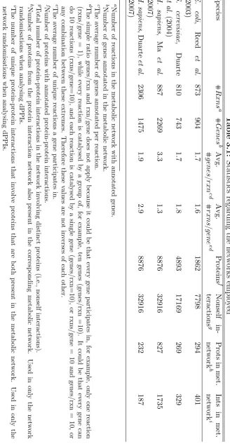
3.1 Statistics regarding the networks employed . . . 48

3.2 Metabolic network structure and dPPI prevalence . . . 55

3.3 More iPPIs in real metabolic networks than in randomised ones 60

4.1 Proportion of self-interacting duplicated genes generated by

different mechanisms . . . 72

4.2 Frequency of self-interaction of singleton and duplicate

(E-value threshold) genes under alternative parameters for

para-log definition . . . 72

4.3 Frequency of self-interactions amongst WGD and SSD

dupli-cate genes under alternative WGD identification methods . . . 72

4.4 Duplicate genes are enriched for self-interactions disregarding

E-value cutoff used to define duplicate genes . . . 74

75table.4.5

4.6 WGD genes are enriched for self-interactions disregarding of

WGD detection method . . . 76

4.7 Over-represented GO terms when self- and non-self-interacting

genes are compared against each other . . . 82

4.8 Over- and under-represented (italics) GO terms when

dupli-cated genes are compared against singleton genes . . . 83

4.9 Over- and under-representation (italics) of GO terms in

List of Tables xv

5.1 Over- and under-represented GO terms of genes present at

least once in a primate-specific PPI . . . 102

5.2 Over- and under-represented GO terms of genes in exclusively

present in primate-specific PPIs . . . 103

5.3 Connectivity statistics for primate and nonprimate genes . . . 104

5.4 Absolute connectivity difference between proteins in primate

and nonprimate PPIs . . . 105

5.5 Co-evolution signal detection using Spearman’s Rank Sums

correlation coefficient ρ comparison of real and pseudo datasets 108

5.6 Over- and under-represented GO terms of genes present in

1.1 Network parameters . . . 3

1.2 Regular, small-world and random network topologies . . . 5

1.3 Power-law distribution . . . 7

1.4 Network distributions . . . 8

1.5 Path length and robustness in scale-free vs random networks . 9 1.6 From metabolic pathway to network depiction . . . 11

1.7 Enzyme and compound centric networks . . . 12

1.8 Network rewiring after WGD . . . 28

1.9 Evolution of metabolic pathways . . . 30

2.1 Different types of gene-protein-reaction associations in yeast metabolic network model iND750 . . . 37

2.2 Cartoon of a metabolic network and how FBA works . . . 41

3.1 iPPIs provide structure to the yeast metabolic network . . . . 56

3.2 iPPIs produce more distinct metabolic subnetworks than expected by chance . . . 59

3.3 Biomass flux and knockdown effects . . . 63

4.1 Data collection . . . 70

4.2 Definition of mouse-specific duplicated genes in human . . . . 71

List of Figures xvii

4.4 Relationship of duplication type and number of interactions . 78

4.5 Number of interactions controlled for age . . . 79

4.6 Distribution of synonymous subsitution rate of WGD and SSD duplicate pairs . . . 80

5.1 PPI presence and absence . . . 91

5.2 Mirrortree with protein-protein interactions . . . 92

5.3 Distribution of correlation coefficients . . . 95

5.4 Datasets used in the GO analyses . . . 99

Abbreviations

AP-MS affinity purification mass spectrometry.

ATP adenosinetriphosphate.

BLAST Basic Local Alignment Search Tool.

BLASTP protein BLAST.

DDC model duplication-degeneration-complementation model.

DIP Database of Interacting Proteins.

dPPI direct protein-protein interaction.

EBI European Bioinformatics Institute.

EC Enzyme Commission.

EHMN Edinburgh Human Metabolic Network.

ER Erd¨os and R´enyi.

FBA flux balance analysis.

FRET fluorescence resonance energy transfer.

FSGD fish-specific genome duplication.

GPR gene to protein to reaction associations.

GSM genome-scale metabolic.

HIV human immunodeficiency virus.

HPRD Human Protein Reference Database.

iPPI indirect protein-protein interaction.

KEGG Kyoto Encyclopedia of Genes and Genomes.

MIPS Munich Information Center for Protein Sequences.

ML maximum likelihood.

MLE maximum likelihood estimation.

MS mass spectrometry.

MSA multiple sequence alignment.

NAD+/NADH nicotinamide adenine dinucleotide.

ORF open reading frame.

PAML Phylogenetic Analysis by Maximum Likelihood.

PGK phosphoglycerate kinase.

PIN protein interaction network.

PPI protein-protein interaction.

SGD Saccharomyces Genome Database.

Abbreviations xxi

TAP tandem affinity purification.

WGD whole genome duplication.

WS Watts and Strogatz.

always been around.’

Chapter 1

Introduction

Once upon a time, scientists who studied proteins spent years studying

a single protein, or a single gene. Their relentless and painstaking

work established the basis of our genetic and biochemical understanding

of cell and organism function, organisation and evolution. Constant

technological development of the methods used on single proteins and genes led to the advent of high-throughput techniques in biotechnology, such as genome sequencing, proteomics and protein interaction identification. The coupling of these methods to computing has enabled the rise of richly populated biological information databases, and the developing science of bioinformatics. A key factor in enabling the development of this field has been to ensure that most data is free and publicly available in databases for anyone to access. This has enabled the possibility for any researcher to move from small-scale to genome-wide studies, and most researchers can now to varying extent use internet based tools to see how their gene or protein of interest, or indeed organism of interest fits into nature’s scheme. Our ability to seek general trends or distinct results in a mass of biological data, rather than being restricted to making extrapolations based on the limited data of a few proteins or a distinct region or system in the cell is helping us learn new things about biology, and discovering new areas of interest that can be further explored. That said, bioinformatics data will probably always need to be qualified by high quality data collected through the patient toil of laboratory researchers.

explore this network’s role in metabolic function. Given that this thesis is about the evolution and function of the genes involved in human protein and metabolic networks, the introductory chapter introduces general features of networks before introducing the specific biological features of biological networks. The same mathematical definition of a network applies just as well to the human protein interaction network as it does to a mobile phone communications or air transport network. Molecular evolution analyses will be used to discuss unique aspects of biological network evolution in terms of the forces acting upon and molecular rates by which genes evolve, and the regulation of gene gain and loss, through gene and genome-wide duplication.

1.1

Brief introduction to networks

A network is represented mathematically as a graph consisting of vertices,

also called nodes (which is how they will be referred to from here on in

this thesis) that are connected to each other through edges (Figure 1.1).

The number of connections each node has to any other node is called the

node’sconnectivity or nodedegree pkq(Albert, 2005). Nodes that are highly

connected in the network (i.e. that have a high k) are referred to as hubs.

Edges in a graph can be directed. In such graphs any edges towards a node are called the node’s in-degree, while any edge leaving the node is called the

node’s out-degree. Clustering coefficient pcq is another network parameter.

Rather than measuring the direct connectivity of a node it measures the interconnectivity of a node’s neighbours. In other words, it measures how well connected the neighbouring nodes of a node are to each other. Other

examples of parameters to quantify a network arepath length (e.g. shortest

and longest) between two nodes in the network. Another parameter is

betweenness centrality, the ratio of the shortest path between two nodes, and the shortest path between the same two nodes passing through a third,

predefined, node (Zhu et al., 2007). There is yet another measure called

closeness centrality, which is the shortest path between a node and all other nodes reachable from it. It can be seen as a measure of how quickly information spreads from one node in the network to all its connecting nodes (Newman, 2008).

Brief introduction to networks 3

k=5

k=2 k=2

k=2

k=1

k=4 k=2

k=1 _k=2

k=1

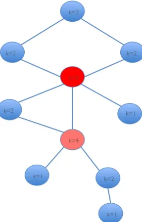
Figure 1.1: Definition of a network and its different parameters.

A network (the mathematical term is a graph) consists ofnodes (depicted as

circles), or vertices as they are also called, and are connected to each other

by edges. The number of connections (connectivity or degree pkq) of each node is written inside of the respective node. Nodes with many connections

i.e. with a high k are called hubs. Here the hub with most connections is

depicted in red (k 5). The pink node, although it does not have as many

connections as the red node, is also a hub (k 4) as it has more connections

than most nodes in the network that are only connected to only one or two

other nodes (k1 ork 2). However, how many connections a node needs

the parameters listed above such e.g., if the network is highly clustered or not. At first it was thought that networks were either regular or random. The regularity of a network is assigned a number between 0 and 1 where

p 0 stands for complete regularity while p 1 means the opposite i.e.

complete disorder. In a regular network every edge (i.e. connection) in the network is evenly distributed causing the path between any two randomly chosen nodes to be very long (as one has to go through many other nodes to get from the first to the second chosen node). Thus making the path length long, and highly clustered. It is said to be a large-world network. In a random network however all the edges are randomly distributed between

the nodes. Thus the random network is a badly clustered, small-world

network. However, Watts and Strogatz (1998) realised that many networks, stretching from technological (such as the power grid in the U.S.A.) and social

networks amongst movie actors to the neural network of C. elegans, were

neither completely regular or completely random, but somewhere in-between

(i.e. with 0   p   1). The topology of these networks was to be called

small-world networks because although most connections between nodes were regular, every now and then a node was highly connected (i.e. a hub), which shortened the path length between two randomly chosen nodes substantially (Figure 1.2). Thus, a network could have mostly regular connections, and only a few ’short-cuts’, and p increased substantially giving the network small-world characteristics of a random network.

Following the discovery of small-world networks in 1998 Barab´asi and

Albert (1999) decided to study the topology and distribution of several large, real (as existing in nature and society rather than generated specifically and artificially for a computational experiment) networks ranging from the World Wide Web to neural networks and protein networks. Previously it

was thought that complex networks were random according to Erd¨os and

R´enyi (ER) graph theory. However, as more network data became available

Barab´asi and Albert could test it, they discovered that none of the data they

tested arranged itself in a way that the ER random graph theory predicted. Further they discovered that real network data did not really conform to the Watts and Strogatz (WS) model describing small-world networks either. Real networks, they realised, obey two very important rules. Firstly, they grew in size as new nodes were added to the network (something neither the ER nor WS model took into account). Moreover, nodes that were already highly

Brief introduction to networks 5

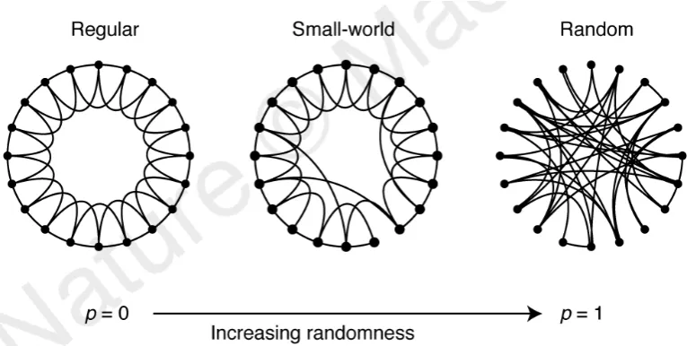
Figure 1.2: Topology of regular, small-world and random neworks.

In the regular network p 0 the edges between the nodes are evenly

distributed. The network is highly clustered and large-world as it would

take long to walk through two randomly chosen nodes. In the random

network p 1 the edges are randomly dispersed between the nodes. Thus,

causing little clustering, and small-world network as moving between two randomly chosen nodes can be very quick. The small-world network lies in-between the two extremes with most edges randomly distributed. However, every now and then edges connect nodes that would otherwise be far apart. Thereby creating ’short-cuts’ in the network, which gives it the small-world

characteristics of the random network. Figure from Watts and Strogatz

and Albert put it the ”rich-get-richer”. It was as though the network kept

re-organising itself into a scale-free state. The degree distribution Ppkq of

a node N is the probability that particular node has k connections, and

is calculated by taking the number of nodes with a particular degree Npkq

divided by the total number of nodesN. Barabasi and Albert realised that

the interactions of the nodes in these networks (i.e., the degree distribution) follow a power-law (Figure 1.3), which can be mathematically expressed

as Ppkq9kγ where 9 stands for ‘proportional to’ and γ indicates how

important hubs are to the network. For example, γ ¡ 3 indicates hubs

are not important, and the network behaves like a random network, while

2 ¡ γ ¡ 3 means there is a hierarchy of hubs i.e. the smaller γ the more

important are hubs to the network (Barab´asi and Oltvai, 2004). Thus, rather

than having the node degree follow the Poisson distribution (Figure 1.4Aa-Ac), which is the case for random networks, the connections of the nodes in these networks follow a power-law distribution (Figure 1.4Ba-Bc) consistent with the fact that most nodes have very few connections, while a few nodes

have very many connections. These networks were calledscale-free networks,

and today we know that there is a range of these network in the real world (which is why they are also sometimes referred to as ‘real-world’ networks)

e.g. the World Wide Web, how authors of scientific papers are cited in

literature, mobile communication networks, several biological networks, such as the protein-protein interactions (PPIs) networks and the neural network

in the brain of several animals (including mammals) (Park and Barab´asi,

2007; Barab´asi, 2009). Compared to regular and random networks scale-free

networks are robust (Figure 1.5). If a node is lost (as long as it is not a highly connected hub) the overall topology will remain intact. In a regular or random network however the loss of any node could disrupt the entire network structure. Also obvious from the same figure is how the longest path length can be substantially shortened in a scale-free network compared to a random network. By passing via a few hubs information can spread very quickly in a scale-free network.

1.2

Biological networks

Biological networks 7

0 50 100 150 200 250

0

500

1000

1500

2000

Power-law degree distribution

No. of interactions (k)

N

o.

o

f p

ro

te

in

s

A

1 2 5 10 20 50 100 200

1

5

10

50

100

500

1000

Log-log plot of the power-law degree distribution

No. of interactions (k)

N

o.

o

f p

ro

te

in

s

B

Figure 1.3: Power-law degree distribution and log-log plot of the same distribution. An example of a real-world, scale-free network is the human protein interaction network investigated in the research chapters of this thesis. Here it is clear that very many proteins have few interactions

while a few proteins have very many interactions. (In this particular

network most proteins only have one interaction, while one protein has 240

interactions.) This relationship of the interactions (degree) a) follows the

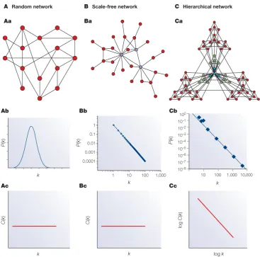
Figure 1.4: Distributions of random, scale-free and hierarchical networks. Figure of networks with their respective node degree distributions

and clustering coefficient distributions plotted below. Aa) A random

network. Ab) The node degree distribution of a random network follows the Poisson distribution. Ac) The clustering coefficient is independent of how many connections a node has. Hence the horizontal line as these two values are plotted against each other onto a graph. Ba) A scale-free network. Bb) Scale-free networks follow a power-law distribution. Bc) Just as for the random network the clustering coefficient is independent from the number of connections of each node. Ca) A hierarchical network. Cb) Hierarchical networks are a type of scale-free networks, which becomes obvious when

the node degree distribution is plotted as it follows the power-law. Cc)

Hierarchical networks are highly clustered, and thus the clustering coefficient is not independent of the node degree. The plot shows how nodes with few connections are highly clustered into separate sections in the network. The different parts of the network are connected to each other by a few hubs.

Biological networks 9

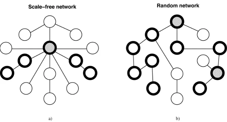
Figure 1.5: Path length and robustness in scale-free vs random networks. Both networks contain the same number of nodes and edges.

a) However, the scale-free network has a hub (grey node) with k 8

connections, and the longest path between any two nodes in the network is 4 steps (see highlighted nodes). b) In the random network two nodes have more connections than the rest, but not by much as their connectivity is

k 3, compared to the connectivity k 1 or k 2 of the remainder of the

functions. It is possible to distinguish between five different types of

biological networks: i) transcription factor binding, ii) protein-protein

interaction (PPI), iii) protein phosphorylation, iv) metabolic interactions and

v) genetic interaction networks (Zhuet al., 2007). This thesis research focuses

on two of these, namely metabolic and PPI networks.

1.2.1

From metabolic pathways to metabolic networks

Metabolism is the biochemical processes whereby the cell’s machinery extracts energy in order to function. The cell builds up complex compounds from simpler ones through anabolism, and degrades complex compounds

into simple sugars through catabolism. One type of protein, enzymes,

catalyse chemical reactions in the cell by lowering the activation energy of a reaction. Thus helping substrates turning into products, which can be consumed by the cell, and/or perform other necessary tasks in the cell’s

metabolism. A reaction where a substrateS is turned into a productP with

the help of an enzymeE can be depicted in a metabolic pathway as follows:

S ÝÑE P, or if the reaction occurs in through several reactions before the

end product is produced as A ÝÑE1 B ÝÑE2 C. Obviously some reactions can

also be reversible, depicted by double-edged arrows. When all the metabolic

pathways in the cell are put together they form a network. A pathway

(Figure 1.6a) can also be depicted as a graph where the nodes are reactions and the edges connecting between the nodes are the substrates (Figure 1.6b). Since some components, such as the co-factors adenosinetriphosphate (ATP) and nicotinamide adenine dinucleotide (NAD+/NADH), are part of very many reactions they are sometimes removed from the network (Figure 1.6c),

and thus a more informative pattern in the network may emerge. Such

components are often referred to as ‘currency metabolites’ (Huss and Holme,

2007). Originally, as the metabolic network depiction evolved from how

metabolic pathways were written, the substrates and products were the nodes while the reactions (i.e. enzymes) where the edges of the network (Figure 1.7a). However, it is now more common to depict the enzymes as the nodes while the reactions are the edges of a metabolic network (Figure 1.7b). Metabolism is modular as many components and enzymes interact only

with a few other components thus forming an isolated group i.e., a module

Biological networks 11

Figure 1.6: From metabolic pathway to metabolic network depiction. Chain of metabolic reactions in a cell depicted: a) In a metabolic pathway b) As a metabolic network where the substrates are the nodes and the reactions connecting these nodes are the edges c) As a simplified metabolic network where co-factors and other promiscuous substrates (often referred to as ‘currency metabolites’) have been removed creating a metabolic network with less nodes. Thus allowing a more informative pattern emerge

Biological networks 13

allows for the reuse of modules through reconnection of interactions between

modules while conserving the interactions within modules. Obviously then

modularity is very important for the evolution of metabolic networks. In fact, metabolic networks are likely to be some of the oldest biological

networks (Caetano-Anolles et al., 2009), as will be further elaborated in

subsection 1.5.2. The modularity makes the metabolic networks hierarchical. As shown in figure 1.4Ca certain networks (e.g., metabolic networks) subdivide into separate modules, which are connected to each other through

a few hubs. Just as for other types of networks the node degree Ppkq follows

the power-law distribution (Figure 1.4Cb), indicating hiearchical networks are scale-free networks. However, the distribution of the clustering coefficient

Cpkq (Figure 1.4Cc) also indicate that the network is highly clustered, and

not independent of the node degree i.e. the number of connections each node

in the network has (Barab´asi and Oltvai, 2004). Ravasz et al. (2002) studied

the properties of 43 different metabolic networks, and concluded that they were all hierarchical, and that this hierarchical modularity corresponded to

distinct metabolic functions of the cell. Since Ravasz et al. (2002) studied

metabolic networks in 43 different organisms it has been proposed that metabolic networks are indeed hierarchically organised (as no metabolic network so far has been found to contradict this statement) i.e. they are

modular. However, they also have a scale-free topology, and thus Cpkq is

independent of the network size, and the degree distribution follows the

power-law (Ravasz et al., 2002; Barab´asi and Oltvai, 2004).

1.2.2

Protein networks

know how they interact with each other in a network we cannot really know all there is to know about each and every protein. As mentioned above the PIN has a scale-free topology, meaning that most proteins have a few interactions, while a few proteins have very many protein interaction partners. They are hub proteins. As illustrated by figure 1.5a if a random node in a scale-free network is removed the main network topology remains intact. However, if the hub is removed the entire network can disintegrate. This might seem fragile, but it actually makes the network much more robust to random loss of nodes. In PINs this is interesting as it has been observed that removal

of highly connected proteins is correlated with lethality (Jeonget al., 2001).

This was further confirmed in a study by Liang and Li (2007) where gene essentiality and protein connectivity was studied in yeast, mouse and human, and where a positive correlation was found between gene essentiality and protein connectivity in both the PIN of yeast and human. As removal of a gene might lead to lethality they realised that whether the gene existed in single-copy or had been duplicated might also correlate to whether or not the gene was essential. They found that highly connected proteins usually exist in a single-copy in yeast, while they have often been duplicated in human. Thus there was a negative correlation between gene essentiality and gene duplicability in yeast, while no such correlation was found in human. Jonsson and Bates (2006) observed that human proteins involved in cancer have many interactions and are central hub proteins in the human PIN.

When Rambaldi et al. (2008) studied this further they further discovered

that not only were genes involved in cancer hub proteins, but that they often only existed in single-copy, and that it was this, rather than their gene function or tissue location, that the cancer genes had in common. Hence, if something happened to a highly connected, single-copy protein this had detrimental effects on the individual as the entire protein network could collapse, affecting far more proteins that those that interacted directly with the affected hub protein.

1.3

Gene gains and losses

1.3.1

Gene duplication

Gene gains and losses 15

and become fixed through genetic drift in small populations than in large ones. Duplicated genes can also undergo positive selection through neo- or

subfunctionalisation. Therefore, certain genes are more likely to become

fixed in a species (thus remaining in the genome) than others. In the study presented in chapter 4 we investigated whether a ‘self-interaction’ (the word refers to when two or more proteins encoded by the same gene interact with each other to form homomers i.e., it is not as in the phosphoglycerate kinase (PGK) example in section 1.4.2 one protein interacting with two parts of itself) plays a role in gene retention after duplication, and whether there is a difference in retention of self-interacting genes that duplicate through small-scale duplication (SSD) compared to genome wide duplication i.e. whole genome duplication (WGD).

1.3.1.1 Factors governing duplicate gene retention

After a gene duplicates the original gene and its newly formed copy can

undergo several different fates. It can gain new, beneficial mutations,

neofunctionalisation, all while the other copy retains the original function of the gene, or both copies can become complementary, and together cover the function of the single ancestral gene - a mechanism called

subfunctionalisation. This last process is explained in the duplication-degeneration-complementation model (DDC model). Originally this model suggested that the two copies of a duplicate pair would subdivide the expression pattern and share the function of the ancestral, single copy gene. According to this model, loss of function will be complementary in the two copies so that both copies are needed to perform the function of the original gene, and therefore the subfunctions must also be independent so that mutations in one gene does not affect functions of the other gene (Lynch

et al., 2001; Papp et al., 2003b; Prince and Pickett, 2002).

allele. Furthermore, it takes longer for a gene to become fixed in a large population compared to a small one. As a consequence a subfunctionalised allele will have more time to gather mutations, which may silence the allele if the mutations are degenerate, but may also save the allele if the new

mutations are benefitial (Lynch et al., 2001).

A recent study suggests that rather than the DDC model after gene duplication the gene and its duplicate copy will first subfunctionalise, then

neofunctionalise, i.e., the duplicate genes will subneofunctionalise. It is

important to consider the effects on the gene network, and not just on the duplicated gene and its newly formed copy. It is more important to stabilise selection, to preserve the ancestral function, than to drive positive selection. The need for stability may explain the high occurence of neofunctionalisation. Moreover, subfunctionalisation in itself is insufficient to explain the high

retention of duplicated genes. Rather, it seems as if gene redundancy

and neofunctionalisation in combination with subfunctionalisation are all important for this retention(MacCarthy and Bergman, 2007).

1.3.2

Whole Genome Duplication

When the entire genome of an organism is duplicated, WGD can occur by two different mechanisms; autopolyploidy or allopolyploidy. In the first case, when the number of chromosomes is doubled within one individual, while in the latter, the fusion of the chromosomes of two nuclei from the parental species where the offspring contains the sum of the parental chromosomes

(Wolfe, 2001; Freeling and Thomas, 2006; S´emon and Wolfe, 2007; Van de

Peer et al., 2009). This leaves three big questions. Firstly, how does an individual that has undergone WGD successfully reproduce unless other individuals of the same species have had their whole genomes duplicated as well? Secondly under what circumstances does WGD occur, and finally what are the biological and evolutionary consequences of WGD?

Gene gains and losses 17

case in polyploid amphibia and fish i.e., the latter can reproduce sexually also as polyploids. When a species has undergone WGD e.g., gone from having its diploid genome duplicated and thus become a tetraploid it can (for many species) successfully reproduce triploid offspring with a diploid individual. The triploid offspring will in turn produce haploid, diploid or triploid offspring (Otto and Whitton, 2000). The problem with polyploid species arose with the sex chromosomes (Wolfe, 2001). Although this problem can be overcome when it is not the X-chromosome (in species with XX / XY sex chromosomes), but rather the presence or absence of an Y chromosome that determines the sex i.e., all of XY, XXY, XYYY, XXYY and XXXY will be male. In birds however (where the female has the sex chromosomes ZW, while the male have two identical sex chromosomes ZZ), ZZW individuals will be of unclear, intersexual phenotype, and mortality will be high. In fact, in a study conducted on chicken none of the eggs with haploid, triploid or tetraploid chromosomes hatched. Human triploid or tetraploid individuals rarely survive until birth. When they do triploid humans are sterile while tetraploid babies do not survive beyond infancy. It is believed that imprinting in mammals is hindering proper growth, which is why there are no adult, polyploid humans (Otto and Whitton, 2000).

Many extant diploid species have polyploid ancestry. However,

poly-ploidization has only prevailed a few times in the evolution of eukaryotic life; Four times in angiosperm, once in fungi, two times in chordate/vertebrates (called 1R and 2R after the first and second rounds of genome duplication)

(McLysaghtet al., 2002; Van de Peeret al., 2010) and a third time in teleost

fish i.e., ray-finned fish (fish-specific genome duplication (FSGD), sometimes also referred to as 3R) (Meyer and Van de Peer, 2005). That is, after a WGD event most genomes will slowly, over millions of years, lose genes until most genes have reverted to the number of loci they had before the WGD event (Conant and Wolfe, 2007). However, these WGD descendants will give rise to great species variety e.g., over 25,000 fish species and over 350,000 flowering plant species. Thus, although many polyploids seem to die before birth, reaching a reproductive age or being sterile, hence unable to reproduce, the few times reproduction is successful it seems to generate evolutionary superior

species (Meyer and Van de Peer, 2005; S´emon and Wolfe, 2007; Van de Peer

genetic variation in order to gain a phenotypic advantage over other diploid species. Hence being able to occupy an ecological niche that has become available due to the dramatic, even cataclysmic ecological changes, while these same polyploid species would not have the same competitive advantage over their diploid sister species in an ecologically stable environment. Several findings support their theory, for example, the FSGD in teleost fish occurred 226 - 316 mya, which overlaps with the Permian-Triassic mass extinction

from 250 mya (Van de Peeret al., 2009). However, this is not the only way

species undergoing polyplodization (i.e. WGD) could gain an advantage over species that had not undergone WGD. Conant and Wolfe (2007) showed that inS. cerevisiae after WGD had occurred all genes in the glycolytic pathway

were retained, which could have givenS. cerevisiae an advantage over other

microbes when sugar-rich fruit appeared on earth, which was around the time of the WGD event in fungi.

1.3.3

Comparisons of Whole Genome Duplication vs

Smaller Scale Duplications

Gene duplication is proposed to occur through SSD or WGD. The latter model of duplication was championed in 1970 by Susumu Ohno (Ohno, 1970). He stated that it is easier to derive new genes through gene duplication than

de novo, and suggested that two or even three rounds of WGD had occurred in vertebrates. As stated in the previous subsection for vertebrates there is now evidence that two rounds of genome duplication (2R) occurred in chordates,

just before and after the divergence of the lamprey lineage (Van de Peeret al.,

2010; Dehal and Boore, 2005), and a third round of genome duplication (3R)

in ray-finned fish (Meyer and Van de Peer, 2005; Van de Peer et al., 2010).

Davis and Petrov (2005) studied gene duplication in the yeastS. cerevisiae.

They found that highly expressed genes are more likely to duplicate, and that orthologues of both SSD and WGD duplicates evolve slower than orthologues of the singleton genes they studied (Davis and Petrov, 2005). Finally they found that SSD and WGD genes differed in their function. WGD genes typically encode catalytic proteins, while SSD genes tend to encode binding proteins and enzymatic regulators, which are rarely found amongst WGD

duplicates. This is consistent with other studies in yeast (Guanet al., 2007;

Hakes et al., 2007a). However, Hakes and colleagues found that although

Gene gains and losses 19

latter are more likely to be essential genes in a protein complex.

Most genes are lost after duplication, regardless of whether the mechanism was small-scale, or genome-wide. A gene duplicated by SSD needs to become fixed in the entire population to be retained. In order for this to happen, the gene usually needs to undergo selection as described above, or the population size must be small to facilitate fixation through random genetic drift. Most duplicates from SSD events never pass this stage. Genes that are duplicated in a WGD event, on the other hand, are duplicated together with all other genes in that individual, which will then undergo immediate speciation, as occurred at the fish-tetrapod split (Dehal and Boore, 2005). Therefore the duplicated genes do not need to become fixed in the genome of the entire

population. However, after a WGD event, the genome will go through

massive genome rearrangement and loss, and many of the duplicated genes will be lost at this stage (Davis and Petrov, 2005; Dehal and Boore, 2005).

1.3.4

Gene dosage and gene duplicability

What forces make a newly duplicated gene prevail in the genome, and become fixed in the population? This question is particularly interesting considering the high loss rate of duplicated genes that follows small-scale or genome-wide duplication events. The answer seems to be due to the gene dosage balance effect. This should not be confused with the gene dosage effect, which occurs when there is not enough gene product in a cell due to the deletion of one of the genes alleles (haploinsufficiency). A gene dosage balance effect refers to the relative dosage of genes whose products interact or function in the same pathway. Qian and Zhang (2008) showed that in human and yeast that there is no statistically significant difference between the duplicability of haploinsufficient and haplosufficient genes i.e. that haploinsufficient genes do not tend to duplicate more often than haplosufficient genes. In yeast they showed that haploinsufficient genes that encode subunits in protein complexes tend to be kept in the genome after a WGD event, supporting

the theory of gene dosage balance effect theory (Papp et al., 2003a; Qian

and Zhang, 2008). Hughes et al.(2007) mention in their review that

dosage-compensations may act as a force, which initially retain duplicate genes

neo-and subfunctionalisation to occur neo-and thereby ensure selection for their

subsequent retention (Hugheset al., 2007; Rastogi and Liberles, 2005). Liang

et al. (2008) studied the protein structure of more than 12 000 proteins, in several species, including human, and showed that proteins that are sensitive to their surroundings for proper folding, called ‘under-wrapped’ proteins (meaning that they are dependent on stabilising interactions from other proteins for their protein structure), are dosage sensitive, and hence more

vulnerable to dosage imbalance (Liang et al., 2008). This in turn makes

duplicate copies of such genes more likely to be lost again after a duplication event. Unless they arose through a WGD event, in which case there will be no gene dosage imbalance since all genes in the organisms genome are duplicated. They also showed that more complex the organisms are less sensitive to gene

dosage imbalance, with E. coli followed by yeast (S. cerevisiae) being the

more sensitive organisms whereas human and thale cress (A. thaliana) were

least dosage sensitive. They found that under-wrapped genes in yeast have a tendency to exist as single-copy genes and not duplicates regardless of their functional category. The correlation between under-wrapped proteins and their decreased gene duplicability appears to be independent of the function of the protein they encode.

1.3.5

How gene duplication affects the protein

inter-action network

Following gene duplication, the proteins of the two newly formed genes should interact with the same set of proteins as the ancestor gene. Asymmetry in the number of PPI partners will arise after the gene pair paralogues have had time to diverge. The two paralogues will each have a different set of interacting partners, and only share a subset of these with their paralogous copy. Makino and Gojobori studied duplicated gene pairs in yeast in order to elucidate whether the dominant evolutionary force is PPI gain or loss. They found that the slower evolving gene copy would have more interaction partners than the faster evolving copy. Moreover when comparing the two copies, they showed that the evolutionary rate difference is smaller in cases where more protein-protein interactions are still shared between the duplicate

pair (Makino et al., 2006; Makino and Gojobori, 2007). Thus while Hahn

Gene gains and losses 21

protein network regardless of the number of PPIs, Makino and Gojobori (2006) showed that interacting paralogous proteins with different functions and in the sparse part of the PIN evolve slower than paralogous proteins in the central part of the PIN and than interacting paralogues with the same function. Liang and Li (2007) investigated the correlation of gene essentiality, gene duplicability and protein connectivity (how well connected a protein is i.e. measure of interacting partners). They found that essential genes in yeast (defined as having a lethal or sterile knockout phenotype) have high protein connectivity and tend to exist in single-copy, and that there is a negative correlation between protein connectivity and gene duplicability. This can be summarized in the ‘central-lethality rule’ meaning that an organism will most likely die if highly connected proteins are deleted. They also investigated these properties in human and mouse, and concluded that highly connected proteins in general have high gene duplicability (that is, the opposite trend), and that despite the presence of duplicates these highly-connected genes are usually essential for the organisms ability to survive or reproduce. No correlation was detected between gene essentiality and gene duplicability (Liang and Li, 2007).

Pereira-Leal and colleagues investigated the evolution of protein com-plexes and concluded that they evolve through the duplication of homod-imers. They showed that protein interactions amongst paralogous proteins occur more frequently than can be expected purely by chance in yeast, worm

and fruitfly (Pereira-Leal et al., 2007). They also show that protein-protein

Pereira-Leal, 2008). Another study shows that 50-70% of proteins with a known quaternary state (i.e., proteins consisting of several polypeptide chains or

subunits (Lenhingeret al., 1993)) form homomers (Levyet al., 2008), which

is not surprising since approximately half of all crystallographic structures

are homo- or heteromeric protein complexes (Levy et al., 2006). Levy et al.

(2008) found that certain quaternary structures, such as dihedral (where the same end of the subunits interact) and cyclic (where the opposite ends of the subunits interact), are more prevalent than other types of structures in homomers. The prevalence of dihedral cases can probably be explained in terms of random mutations not causing disruption to binding between two identical subunits to form a dihedral (since they interact with each other by binding to the same end). In contrast, mutation in a cyclic quarternary structure could disrupt the interaction if a compensatory mutation does not appear in the other end of the interacting subunit. Also, disregarding the forces driving molecular evolution, simply by studying iso-chemical properties of proteins one can conclude that proteins will have a higher affinity for interacting with other proteins which are identical to themselves because the lowest energy distribution of a homodimer is generally lower than that of any

random heterodimer (Lukatsky et al., 2007).

As stated above, it has previously been shown for yeast, worm and fly that paralogous proteins interact more frequently than would be expected

by chance (Pereira-Leal et al., 2007). The same study also showed that

PPIs between homodimers and paralogous dimers in these species are not independent, and that the latter dimer type evolved from the former. Ispolatov and colleagues also showed that duplicated genes tend to self-interact more often than can be expected by chance alone in yeast, worm, fly and human. They also found that the likelihood of a protein self-interacting is proportional to its number of interacting partners, and that proteins forming heterodimers with their paralogues tend to have twice as many interaction partners as the average protein in the network. This lead them to conclude that interactions between paralogous proteins forming heterodimers are inherited from self-interacting proteins which form homodimers and from

Constraints on protein sequences 23

1.4

Constraints on protein sequences

1.4.1

Selection vs genetic drift

When a mutation occurs in a DNA sequence it contributes to the genetic

variation in the population. However, it is not until the substitution is

fixed in the population that the mutation becomes a substitution (Bromham, 2008). Mutations at any given allele do not occur at a high rate in a single

individual. However, if the entire population, of size N, is considered and

if it is a diploid population then there are 2N alleles that can mutate at

rate µ each generation i.e., there are 2N µ mutations per generation in the

population. Thus allowing for great variation within a population (Hartl and Clark, 1997). If the mutation in an individual is passed on to its offspring then the mutation becomes part of the variation in the population (and

we should really be talking about the effective population size Ne i.e., the

individuals in a population that reproduce and hence pass on their mutation to their offspring). Whether the allele is fixed in the population depends on the selective constraints acting upon the allele and on the size of the population ‘harbouring’ the allele in question. If we have the DNA sequence of the allele in question we can detect the selective constraints acting on the allele (and driving it either to fixation or out of the gene pool) estimating

the nonsynonymousKa (also denoteddN) and synonymousKs (also denoted

dS) substitutions per site in the protein coding sequence. As the name

implies nonsynonymous substitutions changes the DNA sequence so that the codon encodes a different amino acid, while a synonymous substitution is silent since it does not change what amino acid is encoded by the codon in the DNA sequence. The ratio of the nonsynonymous over synonymous

substitution rates ω Ka{Ks is called omega, and is a measure of the

selective constraint acting on the protein encoding DNA sequence. If the nonsynonymous mutation gives neither an advantage or disadvantage the nonsynonymous and synonymous mutations will be fixed at the same rate

i.e., Ka Ks and thus ω pKa{Ksq 1. If however the nonsynonymous

mutation is deleterious purifying selection will drive the mutation out of

the population, and Ka   Ks and consequently ω   1. If however

the nonsynonymous mutation is beneficial natural selection will drive the mutation towards fixation (also referred to as adaptive evolution) and hence

in the population will fluctuate under random genetic drift until it is either fixated in or lost to the population. At the beginning of this section we

saw that there are 2N µ mutations in a diploid population of size N. If we

consider that the fixation rate of any one mutation is 1{2N we realise that

for neutral mutations (that are free to fluctuate under random genetic drift since they are not under any selective constraint) the fixation rate is

2N µ

2N µ (1.1)

i.e., the same rate as the mutation rate itself. However, in reality very many mutations are only nearly neutral. Meaning that they have a small effect on fitness, and thus while slightly deleterious mutations would be removed from large populations they could become fixed due to genetic drift in species with small population sizes e.g., mammals (Ohta, 1995), endosymbiotic microorganisms (Woolfit and Bromham, 2003) or species isolated on islands (Woolfit and Bromham, 2005).

1.4.2

Molecular co-evolution and protein interactions

Lovell and Robertson (2010) define molecular co-evolution as ”reciprocal

evolutionary change in evolutionary interacting loci”. This comes from

the original meaning of co-evolution between two species. However, here

it is used to refer to the molecular co-evolution between residues. For

example, if certain residues in a peptide sequence bind to each other for proper protein folding then purifying selection will constrain these sites from mutating if mutation prevents these sites from binding, and ultimately prevents proper folding of the peptide sequence. However, if mutation at one site is compensated by a complementary mutation at the second site then residues can still bind to each other, the peptide sequence can still fold properly and the two sites are co-evolving. This reciprocal change between interacting residues has been studied to identify site-specific co-evolution e.g., for the study of the V3 loop of the human immunodeficiency virus

(HIV) type 1 envelope protein gp120 (encoded by the env gene) using an

entropy approach derived from Shannon’s entropy to identify covarying site

pairs within the loop peptide sequence (Korber et al., 1993). In another

study the entire env gene was scanned for co-evolving residues pairs. 24

Constraints on protein sequences 25

V3 loop, and for the entire gene 848 pairs (consisting of 263 residues) were

found to co-evolve (Travers et al., 2007). However, although 8 residues in

the V3 domain and 5 residues in the co-receptor binding domain of gp120 bind either directly to or within the binding pocket of the host cell’s CD4 receptor, and the method applied (Fares and Travers, 2006) detects co-evolution between pairwise sites detection of co-co-evolution does not necessarily imply an interaction between proteins since also hydrophobicity, molecular weight and the two combined contribute to the co-evolution signal that is

detected (Travers et al., 2007).

Goh et al. (2000) developed a method to predict PPIs using phospho-glycerate kinase (PGK), a two-domain enzyme which is active when the N-and C-terminal bind each other. In order to remain a functional enzyme the two domains must be able to bind to each other, and consequently they must co-evolve since a change in the amino acid sequence of one terminus must be matched by an equivalent change in the other terminus for the binding to be preserved. Therefore PGK was ideal for developing a measure of co-evolution, which could then be used as a standard reference to compare measures from other amino acid sequences thought to bind to each other. Thus, by constructing one multiple sequence alignment (MSA) per terminus, and one phylogenetic tree per terminus of the PGK the correlation coefficient of all pairwise distances between the two trees could be calculated. Then the

overall Pearson’s correlation coefficient, r, was calculated from these values,

and used as a reference when scanning for co-evolution of binding specificity

between chemokine ligands and receptors (Goh et al., 2000).

The method described above was refined in another study where67,000

pairs of E. coli proteins were scanned for co-evolution signal. This was

achieved by constructing MSAs from Basic Local Alignment Search Tool (BLAST) hits and from databases with MSAs. Then for each pair of proteins phylogenetic trees with at least 11 matching branches were constructed i.e. ‘mirrortrees’. Then the correlation coefficient values from known (i.e. real) protein interactions were compared against correlation coefficient values from

the remaining paired proteins. If the correlation coefficient value of two

paired proteins was equal to or higher than that of the protein pairs known to interact it was a good indication that the paired proteins lacking interaction information were indeed interacting as well. Of the 67,209 possible pairs

of protein interactions in E. coli 2742 were predicted to interact using this

were also included in the list of possible protein interactions, and these real PPIs were also predicted to interact using this method. (Pazos and Valencia, 2001).

The mirrortree method has also been applied to detect protein

inter-actions in the eukaryote S. cerevisiae Hakes et al. (2007b). Both Pazos

and Valencia (2001) and Hakes et al. (2007b) report an average of 20%

false positive protein interaction predictions with the mirrortree method. It should also be noted that this method cannot really distinguish between interactions between two proteins, and proteins that are simply members of the same protein complex (Lovell and Robertson, 2010). However, Kann

et al.(2009) successfully identified that although interacting proteins have a co-evolutionary signal along their entire sequence this signal is higher at the binding domain and surrounding binding neighbourhood. Moreover, Tillier and Charlebois (2009) developed a method that measures the strength of co-evolution between any two eukaryotic protein families by finding their largest common distance submatrix. Thus resolving the issue of comparing families of different size and the problem of including paralogous genes into the analysis. Using this method they successfully identified human proteins known to physically interact with each other. Hence distinguishing them from proteins simply belonging to the same biochemical pathway.

The problem with correlated distance methods such as those described above is that nucleotide mutation rates can vary between species. Therefore

if the nonsynonymous substitution rates Ka are normalised against the

synonymous substitution rates Ks by calculating the rate ω pKa{Ksq per

branch (i.e., species), adjustment for the phylogeny is no longer necessary since a species-specific measure was obtained from the rate per branch (Clark and Aquadro, 2010). In fact, Clark and Aquadro found this novel mirrortree method (applied in chapter 5) superior to traditional mirrortree methods (described in paragraph above) that apply pairwise distances to calculate the correlated evolution between pairs of proteins.

1.5

Network evolution

1.5.1

Evolution of protein interaction networks

As mentioned in section 1.1, there are two general characteristics for real

Network evolution 27

attachment (Barab´asi and Albert, 1999), meaning that nodes with many

interactions tend to acquire even more interactions. In a social context, this can be explained by the fact that a person who already has many established contacts will make further contacts through them. On the Internet it makes sense that well established websites are hyperlinked more by other pages, and the more credible sites attract more hyperlinks. In biological networks such as the protein interaction network gene duplication is the explanation for network growth. A duplicate and the original gene are identical immediately after gene duplication. Therefore the two will also share interactions. When a gene encoding a highly connected protein is duplicated the duplicate will also have all the same connections i.e., the number of connections will double. Over time though the original gene and its duplicated copy will start diverging, and consequently their interaction partners might change

(see section 1.3.5) (Barab´asi and Oltvai, 2004; Makino et al., 2006; Makino

and Gojobori, 2007). However, this also explains how the protein network can be rewired and evolve (see section 1.3 and research chapter 4). Several studies have shown that self-interacting genes seem to be a driving force in the

evolution of protein complexes (Wagner, 2001; Ispolatovet al., 2005;

Pereira-Leal et al., 2007; Levy et al., 2008). Indeed Presser et al. (2008) found that

self-interacting genes existed in higher frequency in the ancestral PIN of S.

cerevisiae. Kuninet al.(2004) also studied theS. cerevisiae protein network. They discovered that if they mapped the proteins against an evolutionary tree, and then grouped the proteins according to their connectivity in the network it became clear that proteins involved in similar functions appeared around the same time and had similar number of connections in the network. They observed that the most connected proteins in the network appeared at the time of the eukaryotic lineage suggesting their involvement in the organisation of the eukaryotic cell. Moreover they found that the majority of the oldest, pre-eukaryotic proteins had few connections and were metabolic enzymes, consistent with the fact that metabolism is a very old mechanism indeed.

Figure 1.8: Rewiring of a PIN after WGD.Rewiring of a protein network after

WGD: All proteins in a

PIN are duplicated through WGD. Hence, initially all the edges (PPIs) are also

dupli-cated. However, with time

some interactions between

Network evolution 29

1.5.2

How metabolic pathways and networks evolve

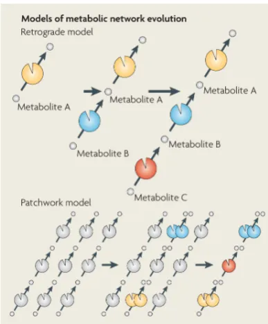
There are several theories on how metabolism and metabolic pathways

evolved. The first one is called retrograde evolution (Horowitz, 1945). As

the name suggests the hypothesis proposes that metabolic pathways evolved

backwards. That is, at first there is plenty of a particular metabolite A,

which is necessary for an organism to survive. With time, however, this metabolite is depleted, giving an advantages to organisms with an enzyme

E1 capable of producing metabolite A from another metabolite B :B ÝÑE1 A

(Figure 1.9; retrograde model). Then as metabolite B is also depleted

an organism where enzyme E1 has duplicated and diverged to E2 will be

able to recruit metabolite C in order to produce metabolite B, and finally

produce the essential metabolite A:CÝÑE2 B ÝÑE1 A. However, the retrograde

evolution model requires an abundance of substrates, ready to be used, which is not a very likely scenario considering that many intermediate metabolites are unstable. Therefore, in 1974 Ycas proposed, and two years later Jensen

expanded on, another hypothesis called patchwork evolution (Ycas, 1974;

Jensen, 1976). This model suggests that in the early days of metabolism organisms with broad-spectrum enzymes could gain an advantage over other organisms as their enzymes could produce a wide number of new metabolites,

and new metabolic functions could thus evolve. However, through gene

duplication and subsequent sub- and/or neofunctionalisation the enzymes became specialised. Although the new specialised enzymes are not capable of catalysing many different substrates they are very efficient in catalysing one substrate