3-D Visualization and Optimization of
Input-Output Relation for Linear Systems Using
Parametrization of Two-Stage Compensator Design
Kazuyoshi MORI
Keisuke HASHIMOTO
Abstract—In this paper, we consider the two-stage com-pensator designs. As an investigation of the characteristics of the two-stage compensator designs, which is not well in-vestigated yet, we implement three dimensional visualization systems of input-output relation and optimization system of the parametrization of stabilizing controllers based on the two-stage compensator design.
Index Terms—Linear systems, Feedback stabilization,
Visu-alization, Two-Stage Compensator Design, Mathematica
I. INTRODUCTION
I
N this paper, we consider the two-stage compensator designs in the framework of the factorization approach. In the design, during the first stage, a new closed loop system selects stabilizing compensator for the plant. In the second stage, a stabilizing controller is selected for the new closed-loop system that also achieves some other design objectives such as decoupling and sensitive minimization.Recently, we have given a parametrization of stabilizing controllers of the two stage compensator design based only on the factorization approach, which is in the form of the Youla-Kuˇcera-parametrization[1], [12], [13], [14].
The factorization approach to control systems has the ad-vantage that embraces, within a single framework, numerous linear systems such as continuous-time as well as discrete-time systems, lumped as well as distributed systems, one-dimensional as well as multione-dimensional systems, etc[1], [2], [3]. Hence the result given in this paper will be able to a number of models in addition to the multidimensional systems. In the factorization approach, when problems such as feedback stabilization are studied, one can focus on the key aspects of the problem under study rather than be distracted by the special features of a particular class of linear systems. This approach leads to conceptually simple and computationally tractable solutions to many important and interesting problems[4]. A transfer matrix of this approach is considered as the ratio of two stable causal transfer matrices. In some design problems, one uses a so-called two-stage compensator design for selecting an appropriate stabilizing compensator. One of examples of two-stage compensator design is earthquake-resistant dumpers for a building shown in Figures 1. Another example of two-stage compensator design is earthquake-resistant dumpers for a bridge shown in Figures 1. By attaching resistant dumpers to these building and bridge, these building and bridge become strong against earthquake.
Manuscript received March 18, 2016; revised April 6, 2016.
[image:1.595.307.546.199.378.2]K. Mori and K. Hashimoto are School of Computer Science and Engi-neering The University of Aizu, Aizu-Wakamatsu 965-8580, JAPAN email: [email protected].
[image:1.595.306.546.421.602.2]Fig. 1. Earthquake-Resistant Dumpers for building.
Fig. 2. Earthquake-Resistant Dumpers for bridge.
C
P
u
2 [image:2.595.347.503.55.197.2]u
1e
1y
1e
2y
2Fig. 3. Feedback systemΣ.
To achieve this, we have implemented visualization sys-tems of the parametrization of stabilizing controllers based on the two-stage compensator designs [16], [17], [18] and also implemented system, which present norms of output signals and optimize the system based on the two-stage compensator design. We call these system Visualization system and Optimization system, respectively.
In Visualization system, output signals can be visualized as 3D graphs. Because we use Mathematica, we can overlook output signal with all parameter by using some implemented functions of 3D graph system such as we can rotate 3D graph by dragging the mouse inside the graphic. In Optimization systems, norms of output signals can be visualized 3D graphs and minimum norm of output signals can be found by Golden Section Method[15].
In this paper, we consider the SISO and MIMO discrete-time LTI systems as a model of the factorization approach.
II. PRELIMINARY
The stabilization problem considered in this paper follows the papers [6], [7], in which the feedback systemΣ[4] is as in Figure 3. For further details the reader is referred to the literatures[4], [6], [7], and [8].
We consider that the set of stable causal transfer functions is an integral domain, denoted by A. The total ring of fractions of Ais denoted by F; that is, F ={n/d|n, d∈ A, d6= 0}. This F is considered as the set of all possible transfer functions, which is given as ratio of two stable causal transfer functions. Matrices over F are transfer matrices. Let Z be a prime ideal of A with Z 6= A. Define the subsets P andPs ofF as follows:
P = {a/b∈ F |a∈ A, b∈ A\Z},
Ps = {a/b∈ F |a∈ Z, b∈ A\Z}.
Then, every transfer function in P (Ps) is called causal (strictly causal). Analogously, if every entry of a transfer matrix is in P (Ps), the transfer matrix is called causal (strictly causal).
In this paper, we consider the discrete-time LTI system, then
A = {u
v |u, v∈R[d], all rootsrofv are with|r|>1},
Z = (d),
dis the unit delay operator.
Throughout the paper, the plant can be either SISO or MIMO, and its transfer function, which is also called aplant itself simply, is denoted byP and belongs toPn×m
, which means that the plant has m inputs andn outputs. We can always represent P in the form of a fraction P = N D−1, whereN ∈ An×m
andD∈ Am×m
[image:2.595.91.248.60.104.2]with nonsingular.
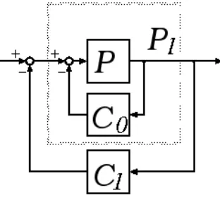
Fig. 4. Two-Stage Compensator Design (y2 tou2).
For P ∈ Fn×m
and C ∈ Fm×n
, a matrix H(P, C) ∈ F(m+n)×(m+n)is defined as
H(P, C) :=
(In+P C)
−1 −P(I
m+P C)
−1
C(In+P C)
−1 (I
m+P C)
−1
(1)
provided that In +P C is a nonzero of A. This H(P, C)
is the transfer matrix from ut
1 u
t 2
t
to et 1 e
t 2
t
of the feedback systemΣ. If In+P C is a nonzero ofA and H(P, C) ∈ A(m+n)×(m+n), then we say that the plant P isstabilizable,P is stabilized by C, and C is a stabilizing controller ofP. In the definition above, we do not mention the causality of the stabilizing controller. However, it is known that if a causal plant is stabilizable, there is always a causal stabilizing controller of the plant [7].
We will denote byS(P) the set of stabilizing controllers ofP.
The following is well known Youla-Kuˇcera-parametrization(Theorem 1)to provide the set of all stabilizing controllers.
Theorem 1: ([1], [12], [13], [14]) Let P denote a causal plant of Pn×m
. LetP =N D−1 = D˜−1N˜. Select X˜,Y˜,X andY such that
˜
Y N+ ˜XD=Im, N Y˜ + ˜DX =In. (2)
Then the S(P) is given by
S(P)
= {( ˜X−RN˜)−1( ˜Y +RD˜)|R∈ Am×n
,|X˜−RN˜| 6= 0}
= {(Y+RD)(X−N R)−1
|R∈ Am×n
,|X−N R| 6= 0},
whereRis a parameter matrix.
III. TWO-STAGECOMPENSATORDESIGN
The two-stage compensator design is for selecting an appropriate stabilizing compensator[4]. Given a plantP, the first stage consists of selecting a stabilizing compensator for P. Let C0 ∈ S(P) denote a compensator of P (that is, an arbitrary but fixed compensator of P) and define
Fig. 5. Composite Stabilized Feedback withc0andc1.
Theorem 2 is same as Theorem 5.3.10 of [4]. Theorem 3 is a generalized version of Theorem 2 with coprime factor-izability. We will employ following theorems and corollary to achieve two stage compensator design.
Theorem 2: ([5]) Let P denote a causal plant of Pm×n
and C0 a causal stabilizing controller of P (C0 ∈ Pm×n). Further let P1 beP(Im+C0P)−1. Denote byC0+S(P1) the following set:
{C0+C1|C1∈ S(P1)}.
Then
C0+S(P1)⊂ S(P), (3)
[image:3.595.94.244.63.182.2]with equality holding if and only if C0∈ Am×n.
Figure 4 cannot implement all controllers as the stabilizing controllers in general.
Theorem 3: ([5]) LetP,C0,P1 be as in Theorem 2. Let N, D,N˜,D˜,Y,X,Y˜, X˜ be matrices over Asuch that
P =N D−1= ˜D−1N ,˜ C
0=Y X−1= ˜X−1Y ,˜ ˜
Y N+ ˜XD=Im, N Y˜ + ˜DX =In.
Then,
C0+S(P1) = {( ˜X−RN˜)−1
( ˜Y +RD˜)|R= ˜XR1X, R1∈ Am×n} = {(Y+RD)(X−DR)−1|R= ˜XR
1X, R1∈ Am×n}.
We can obtain Theorem 3 by replacing parameter R of Theorem 1 withXR˜ 1X.
By Theorem 2, we see that the sum ofC0and a stabilizing controller of P1, say C1, is again a stabilizing controller of
P. This sum, a stabilizing controller of P, is the parallel allocation ofC0 andC1, as shown in Figure 5.
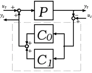
The theorems were based on the feedback fromy2 tou2 (cf. Figures 3 and 4). Even so, we note that, from Figure 3, we have two inputs u1 and u2 and two outputs y1 and
y2. Thus we can consider alternative two-stage compensator design based on other input(s) and other output(s). Let us consider the two-stage compensator design based on the feedback fromy1 tou1. In this case, the feedback system is as in Figure 6.
The configuration is as in Figure 7.
Based on this feedback, the following result has also been given in [5].
Corollary 1: ([5]) LetP,C0,P1 be as in Theorem 2. Let
N,D,N˜ ,D˜ ,Y,X,Y˜,X˜ be as in Theorem 3.
Fig. 6. Feedback fromy1 tou1.
Fig. 7. Composite Stabilized Feedback withc0andc1based on Feedback
fromy1 tou1.
Then we have,
C0+S(P1)
= {( ˜X−RN˜)−1( ˜Y +RD˜)|
R=−Y R˜ 2Y, R2∈ An×m,|X˜ −RN˜| 6= 0} = {(Y+RD)(X−N R)−1|
R=−Y R˜ 2Y, R2∈ An×m,|X−N R| 6= 0}.
We can obtain Corollary 1 by replacing parameter R of Theorem 1 with Y R˜ 2Y where R2 of Corollary 1 is equal toRof Theorem 1.
IV. DEMONSTRATION
Due to the space limitation, we present here the SISO plant case only. As an example, we considerP as follows:
P = d
2+ 1
d2−1 2d+
1 4
,
and the inputs u1 and u2 be 0 and 1, respectively, where
d denotes the delay operator. In this case, the coprime factorization is given as
N =Ne = 16 25(d
2+ 1), D=De = 4
25(2d+ 1) 2,
Y =Ye =7
4 +d, X=Xe =− 3 4 −d.
We consider two constantsa andb and the forma+bd
as a parameter.
[image:3.595.355.497.224.342.2] [image:3.595.338.534.669.709.2]Fig. 8. 3D graph animation of output signaly1based on Theorem 3.R1
form isa+bd.aandbrange are−20≤a, b≤20.
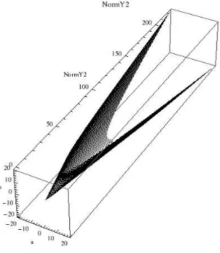
Fig. 9. 3D graph animation of output signaly2based on Theorem 3.R1
form isa+bd.aandbrange are−20≤a, b≤20.
In these visualization, the constant a is implemented by Slider Function of Mathematica. On the other hand, the constantb is one of three axes. Thus the figure changed by time (the value of the constanta), so that they are animations on Mathematica.
Next, we consider l2-norms of signals. Again let −20≤
a, b ≤ 20, R1 = a+bd, u1 = 0, and u2 = 1. Then the norms of y1 and y2 based on Theorem 3 are visualized as Figures 12 and 13, respectively. Also the norms of y1 and
y2based on Corollary 1 are visualized as Figures 14 and 15, respectively.
Minimum norms based on Golden Section Method[15] are shown in Table I.
Figure Minimum norm Figure 12 1.60389 Figure 13 1.29109 Figure 14 1.94602 Figure 15 1.56893
TABLE I
MINIMUM NORM OFFIGURES12TO15.
Fig. 10. 3D graph animation of output signaly1based on Corollary 1.R2
form isa+bd.aandbrange are−20≤a, b≤20.
Fig. 11. 3D graph animation of output signaly2based on Corollary 1.R2
form isa+bd.aandbrange are−20≤a, b≤20.
Fig. 12. Norms of output signaly1based on Theorem 3.R1form isa+bd.
Fig. 13. Norms of output signaly2based on Theorem 3.R1form isa+bd.
[image:5.595.48.216.317.496.2]aandbrange are−20≤a, b≤20.
Fig. 14. Norms of output signaly1 based on Corollary 1. R2 form is
a+bd.aandbrange are−20≤a, b≤20.
Fig. 15. Norms of output signaly2 based on Corollary 1. R2 form is
a+bd.aandbrange are−20≤a, b≤20.
V. CONCLUSION ANDFUTUREWORKS
In this paper, we have visualized the input-output relation for discrete-time LTI systems using parametrization of two-stage compensator design. We also visualize the norms of the outputs and obtained the optimization by using the golden section method.
We consider that the optimization by golden section method is to obtain the minimal or maximal values numeri-cally, which is not theoretical. We will investigate the method to obtain the optimal values by theoretical method.
REFERENCES
[1] C. A. Desoer, R. W. Liu, J. Murray, and R. Saeks, “Feedback system de-sign: The fractional representation approach to analysis and synthesis,”
IEEE Trans. Automat.Contr., vol. AC-25, pp. 399-412, 1980. [2] M. Vidyasagar, H. Schneider, and B. A. Francis, “Algebraic and
topo-logical aspects of feedback stabilization,”IEEE Trans. Automat. Contr., vol. AC-27, pp. 880-894, 1982.
[3] K.Mori, “Parametrization of all strictly causal stabilizing controllers,”
IEEE Trans. Automat. Contr., vol. AC-54, pp.2211-2215, 2009. [4] M. Vidyasagar, Control System Synthesis: A Factorization Approach,
Cambridge, MA:MIT Press, 1985.
[5] K. Mori, “Multi-stage compensator design -a factorization approach-,” inProceedings of The 8th Asian Control Conference(ASCC 2011), 2011, 1012-1017.
[6] V. R .Sule, “Feedback stabilization over commutative rings: The matrix case,”SIAM J. Control and Optim., vol. 32, no. 6, pp. 1675-1695, 1944. [7] K. Mori and K. Abe, “Feedback stabilization over commutative rings: Further study of coordinate-free approach, ” SIAM J. Control and Optim., vol. 39, no. 6, pp. 1952-1973, 2001.
[8] S. Shankar and V. R.Sule, “Algebraic geometric aspects of feedback stabilization,” SIAM J. Control and Optim., vol. 30, no. 1, pp. 11-30, 1992.
[9] P. Wellin,Programming with Mathematica:An Introduction, Cambridge University Press, 2013.
[10] ThreeDimensionalSurfacePlots:http://reference.wolfram.com/ mathe-matica/tutorial/ThreeDimensionalSurfacePlots.en.html.
[11] S. Wolfram, “The Mathematica Book Forth Edition,”Wolfram Re-search, Inc.
[12] F. A. Aliev and V. B. Schneider, “Comments on Optimizing Simul-taneously Over the Numerator and Denominator Polynomials in the Youla-Kucera Parameterization”IEEE Trans. Automat. Contr., vol. 52, no. 4 pp. 763, 2007.
[13] D. C. Youla, H. A. Jabr. and J. J. Bongiorno, “Modern Wiener-Hopf design of optimal controllers Part II: The multivariable case,” IEEE Trans. Automat. Contr., vol. AC-21, no. 3 pp. 319-338, Jun. 1976. [14] V. Kuˇcela, “Stability of discrete linear control systems,”Preprintsc 6th
IFAC World Congr., Boston, MA, 1975.
[15] W. H. Press, S. A. Teukolsky, W. T. Vetterling and B. P. Flannery, “NUMERICAL RECIPES THIRD EDITION: Golden Section Search in One Dimension,”Cambridge university, pp. 492-495, 2007. [16] K. Hashimoto and K. Mori, “Visualization Input-Output Relation with
Parametrization of Two Stage Compensator Design”, The Society of Instrument and Control Engineers Tohoku Chapter., Japan, Fukushima, no. 284-7, Nov. 2013.
[17] K. Hashimoto and K. Mori, “Visualization of The Input-Output Relation of Multi-Input Multi-Output System Using Parametrization of Two-Stage Compensator Design”,Tohoku-Section Joint Convention of Institutes of Electrical and information Engineers, Japan, Yamagata, no. 2F01, Aug. 2013.
[18] K. Hashimoto and K. Mori, “VISUALIZATION OF THE INPUT-OUTPUT RELATION OF SINGLE-INPUT SINGLE-INPUT-OUTPUT SYS-TEM AND MULTI-INPUT MULTI-OUTPUT SYSSYS-TEM USING PARAMETRIZATION OF TWO-STAGE COMPENSATOR DESIGN”,
[image:5.595.55.212.565.745.2]