18
A New Makespan Estimation Model for Scientific
Workflows on Heterogeneous Processing Systems
D. Sirisha
Department of
Computer Science and
Engineering, Pragati Engineering College,
Surampalem, India
G. Vijayakumari
Department of Computer Science and
Engineering, JNTUH College of Engineering,
JNTU, Hyderabad, India
ABSTRACT
Scientific workflows epitomizing computation-intensive applications demand heterogeneous processing resources for attaining high performance. Generally, optimal scheduling of the tasks in workflow is well-acknowledged NP-complete problem. In the present work, a new makespan estimation model is proposed to estimate the bounds on the makespan of the workflows using minimal information. The performance of the proposed estimation model is evaluated using four scientific workflows and the estimation of the makespan computed by the model is compared with the actual makespan generated by the most-cited heuristic scheduling algorithms devised for heterogeneous processing systems. The experimental results revealed that the proposed estimation model is effective and can precisely estimate the makespan of the workflows with an error of over 10% and 26% for computation-intensive and data-intensive workflows respectively.
General Terms
High Performance Computing, Workflow Scheduling, makespan estimation
Keywords
scientific workflows; high performance; heterogeneous processing resource; makespan; makespan estimation
1.
INTRODUCTION
Large monolithic applications in numerous scientific fields such as knowledge discovery, bioinformatics, computations, weather and climate modeling, earthquake science, genome analysis and astronomy can be broken down into smaller tasks structured with intricate dataflow dependencies among themselves are often structured as scientific workflows. Scientific workflows expedite scientists to nimbly model the computation intensive applications as multi-stage computational tasks usually involving a series of data processing operations such as data retrieving, transformation, analysis and aggregation stages. The complexity and the heterogeneity of the scientific workflows demands Heterogeneous Processing Resources (HPR) to attain high performance. HPR are the most potential platforms for rendering high performance at lower costs.
The contributions of the current work are
A new makespan estimation model is proposed to estimate the bounds on the completion time, i.e., makespan of the scientific workflows.
The proposed model estimates the Best-Case Computation Time (BCCT) and Worst-Case Computation Time (WCCT) of the scientific workflows using minimal information.
The computational complexity of the new makespan estimation model is lesser than the existing models.
Validation of the model is performed with the most-cited heuristic scheduling algorithms developed for HPR.
In general, workflow scheduling problem is a well-acknowledged NP-Complete problem [1]. However, the available estimation models deal with simple workflows having unit tasks and no dataflow latencies. Hence, the existing models are not viable for scientific workflows. The proposed estimation model is devised using minimal information, i.e., the profile of the scientific workflows. Generally, the profile of the scientific workflowsconstitutes of the height and the parallelism of the workflow. As the makespan of the workflow highly depends upon the profile of the workflows, these two parameters chiefly contribute for devising good and precise makespan estimation model which can satisfy all the cases.
A makespan estimation model is valid only when BCCT and WCCT functions are admissible. The admissibility of the estimating functions must guarantee that the BCCT never overestimates and WCCT never underestimates the actual makespan of the scientific workflow. Therefore, the estimation model must provide tight bounds on the makespan. The primary aim of the new makespan estimation model is to provide a-priori information of the bounds on the makespan i.e., BCCT and WCCT of the scientific workflows. The a-priori information provided by BCCT and WCCT bound is required to schedule the workflows, provide the resources, and guides in devising the scheduling algorithms.
The remaining paper is structured as follows. In section II, the problem is described, and the overview of the scientific workflows is illustrated in section III. In section IV, the related work is detailed and in section V, the new makespan estimation model is presented. In section VI, the proposed model is evaluated using four scientific workflows and finally section VII summarizes the present work.
2.
PROBLEM
DESCRIPTION
2.1
Application Model
non-19 negative integer di,j that denotes the dataflow time between the
tasks ti and tj. A task having no
[image:2.595.104.242.125.448.2]
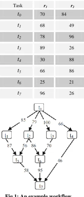
Table 1. Computation Time Matrix
Fig 1: An example workflow
predecessor is termed as the start tasktstart and the task with no successor is the sink task tsink. Generally, a workflow includes a start task and a sink task otherwise a pair of pseudo start, and sink tasks must be connected with pseudo edges to the numerous start and sink tasks. The matrix D of order n × n
is used to represent the dataflow time between the tasks, where each element di,j in the matrix D indicates the dataflow time between the tasks tiand tj.
The organization of the tasks in a workflow describes the structure of the workflow. A task happens to be free upon the completion of all its predecessors and after it receives the data from its predecessors it becomes ready. As each task becomes
ready it is placed in the queue for execution. An example workflow is shown in Figure 1.
2.2 HPR Model
A HPR model constitutes of a suite of m resources < r1, r2...rm > ∈ R with varied processing potentials, fully connected with high speed network. Each resource can execute only one task at a time i.e., tasks cannot be preempted. The execution of task tj and its predecessor ti on the same resource, i.e., r(ti) =
r(tj), then the dataflow between the two tasks is assumed as
local and dataflow time di,j is zeroed. Since, the output data generated by the task ti is available at the same resource on which task tj is to be performed, transferring of the data is not required. Otherwise, i.e., r(ti) ≠ r(tj), the dataflow is assumed to be remote. Moreover, the computations of the tasks and the dataflow between the tasks are carried out simultaneously. The matrix E of order n × m is used to represent the
computation time of n tasks on m resources and each element
wi,j denotes the computation time of the task ti on resource rj. Table. 1 shows the computation time matrix for the workflow depicted in Figure 1.
The key attributes required to describe the workflow scheduling are the Earliest Start Time (EST) and the Earliest Completion Time (ECT). The EST and ECT of the task ti on resource rj are denoted as EST(ti,rj) and ECT(ti,rj) respectively and computed by (1) and (2) respectively. The EST for a start task tstart is zero.
EST(ti,rj) = max { ready(ti), avail(rj) } (1)
ECT(ti,rj) = EST(ti,rj) + wi,j (2) where ready(ti) is the time the task ti becomes ready and
avail(rj) is the time the resource rj is available to execute the next task. In the equation (2), ECT(ti,rj) is computed by
EST(ti,rj) and wi,j, where wi,j is the computation time of the task
ti on resource rj. The schedule length, i.e., makespan of W is the Actual Completion Time (ACT) of tsink, given by (3)
makespan = ACT(tsink) (3)
Definition 1 (Bottom Level). The bottom level of task ti is the length of the longest path from the task ti to tsink. It is denoted as bl(ti) and computed by the computation and dataflow times along the path using (4)
bl(ti ) = w + maxi tj ∈ succ(ti){ bl(tj) + di,j } (4)
where w i is the average computation time of the task tiand
succ(ti) is a set of immediate successors of tiand di,j is the
dataflow times between the tasks ti and tj.
Definition 2 (Top Level). The top level of the task ti is the length of the longest path from the start task tstart to ti, excluding the computation time of ti. It is denoted as tl(ti) and computed by the computation and dataflow times along the path using (5)
tl(ti ) = maxtj ∈ pred (ti){ tl(tj) +wj + dj,i } (5)
where pred(ti) is a set of immediate predecessors of ti and dj,i
is already explained in the equation (4).
Definition 3:The Critical Path (CP) is the longest path in the workflow and the length of the CP can be computed by the sum of the computation and dataflow times along the path and denoted as CPl. The computation critical path is computed by the sum of the minimum computation time of each task on CP, it is denoted as CPc and computed using (6).
CPc = ti ∈ CP min r ∈ R wi (6)
The CP tasks in a workflow can be identified by summing up
bl(ti) and tl(ti) for each task ti. All the tasks on CP have same (bl(ti) + tl(ti)) value which is equal to CPl.
3.
THE
RELATED
WORK
Limited research work has been carried out in estimating the performance of the workflows.
Fernandez et al. [4] were the first to devise lower bounds on the makespan for the workflows with unit sized tasks having no dataflow latencies and performed on homogeneous environments. To compute the lower bound, an interval [θ1,θ2] during which maximum number of tasks n' ⊂ n can be executed is considered such that [θ1,θ2] ⊂ [0, CPc]. For m resources, and n tasks in the workflow, then m × (θ1− θ2)
Task r1 r2
t
0 70 84t
1 68 49t
2 78 96t
3 89 26t
4 30 88t
5 66 86t
6 25 2120 denotes the tasks executed on m resources. The excess area is
divided by m and added to CPc.
The WCCT, i.e., the upper bound of the workflow was first proposed by Jain et al. [5]. The computation of the upper bound was confined to the workflows consisting of unit computation time tasks having no dataflow overheads and was executed on homogeneous systems. The workflow is partitioned according to the levels and the upper bound for each partition was computed by the summation of the number of ready tasks divided by m. Finally, the upper bounds of all
the partitions are summed up to obtain the upper bound of the workflow. Moreover, the lower bound is computed by considering a partition in which the maximum number of tasks can be executed and is divided by m.
In [8], a level based estimation model is proposed to analyze the computation times of the workflows. The model requires the workflow to be partitioned into levels in both top-down and bottom-up approaches to group the set of tasks which can be performed concurrently. The level computation time is computed by the sum of the computation times of all the tasks
[image:3.595.71.497.203.593.2]
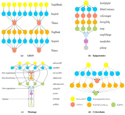
Fig 2: The structure of the scientific workflows
in a level. The makespan for each level is computed by the maximum of the level computation time divided by m and the maximum computation time of a task at that level. The performance of the workflow is estimated by the summation of the makespan of all the levels and nominal dataflow latency is added to it.
4.
AN OVERVIEW OF SCIENTIFIC
WORKFLOWS
Generally, scientific applications are categorized as computation-intensive, data-intensive, memory -intensive, or a combination of these based upon the applications. The computation-intensive workflows consist of tasks which expend most of the time in computations, while the tasks in the data-intensive workflows generate enormous data and
therefore involve much in exchanging data rather than computations [6]. The tasks in the memory-intensive workflows demand high physical storage requirements. Most of the scientific applications embrace workflows to epitomize computation- intensive applications for efficient computation on heterogeneous environments which are the most preferred platforms for attaining high performance.
Laser Interferometer Gravitational Wave Observatory (LIGO) is an Inspiral Analysis Workflow [11]. LIGO is a memory bound and heavily computation-intensive workflow that detects gravitational waves generated by numerous events in the universe according to Einstein’s theory of relativity. The LIGO workflow structure allows greater parallelism. This workflow is applied to analyze the data acquired by
(a) LIGO (b) Epigenomics
21 amalgamating of compact binary systems, namely binary
neutron stars and black holes. The time-frequency data from any event for each of the three LIGO detectors is fragmented into small chunks and then analyzed. A set of waveforms which belong to the parameter space are generated for each chunk. Matched filter output is computed and triggers if Inspiral is detected which are then tested for consistency by the Thinca jobs. Inspiral jobs are highly computation-intensive. Trigger output generates Template banks. The structure of the LIGO workflow is depicted in Figure 2(a).
Epigenomics [12] is a computation-intensive and largely data parallel pipelined application. This workflow primarily processes pipelined data to execute genome sequence jobs which is utilized by Maq system. The remaining jobs of the workflow include filter of noise and contaminated data, a map job which aligns the current location in a reference genome, which is mostly computation-intensive and generates global map to identify the sequence density at each position in the genome. A simple way to enhance performance is to run Epigenomics on heterogeneous platforms since many tasks of this application can run in parallel and are heterogeneous and the structure of this application is given in Figure 2(b).
Montage workflow is devised by NASA / IPAC [9] is an astronomical image mosaic engine which is more widely studied workflow applications. Montage is designed to take multiple astronomical images from telescopes or any other instruments and amalgamate into a single mosaic that appears to be taken from a single instrument. The input images are re-projected onto a sphere and the overlap of the images is calculated. Subsequently, the images are re-projected to correct the orientation and to normalize the background. Lastly, all the processed images are composed into a single mosaic. Astronomers can tailor the functionalities of Montage workflow and add code according to the requisites. Accordingly, Montage is designed consisting of a set of tasks and mostly, the tasks spend much time in communicating and very lesser amount of time in the computation and hence Montage is described as data-intensive workflow and its structure is shown in Figure 2(c).
Cybershake is a seismological application which is highly data and memory-intensive and its structure is depicted in Figure 2(d). This application is generated by the Southern California Earthquake Center [10] to characterize earthquake hazards in geographical regions using Probabilistic Seismic Hazard Analysis (PSHA) technique. The application utilizes Earthquake Rupture Forecast (ERF) to detect the probable ruptures within 200km of an interested region. For every rupture, rupture definitions are converted from ERF into numerous rupture variations with varying hypocenter positions and slip time distributions to generate Strain Green Tensors (SGT). Subsequently, synthetic seismograms for every rupture variation are computed and peak intensity measures are derived from the synthetics which are then combined with the original rupture probabilities to generate probabilistic seismic hazard curve in the region. The information provided by PSHA is utilized by city planners and building engineers to estimate seismic hazards prior to construction of the buildings.
5.
A
NEW
MAKESPAN
ESTIMATION
MODEL
Basically, the makespan of the workflow is influenced by the profile of the workflow, dataflow latencies between the tasks in the workflow and the number of resources employed in the computation of the workflow.
The profile of the workflow includes the implicit parallelism and the height of the workflow. The execution of the parallel tasks concurrently on an adequate number of resources can significantly reduce the makespan. On the other hand, the height of the workflow reflects the longest path in the workflow, i.e., the CP. Because of the sequential bottlenecks of the CP tasks, these tasks can only be performed serially and hence provisioning of additional resources may not further minimize the makespan.
The main shortcomings of the existing models in the literature are they do not consider the dataflow latencies among the tasks and hence do not fit for the scientific workflows. On the other hand, the new makespan estimation model is devised considering the Critical Path (CP), and the intrinsic parallelism of the workflow. The proposed estimation model captures the workflow parallelism by effectively identifying the independent branches in a workflow. CP is a global heuristic and the inherent sequential path of the workflow that plays a pivotal role in determining the bounds on the computation time.
Theorem 1:Let W = <T,E,w,d> be a workflow and CPc be
the compute critical path. For any schedule S of W, the makespan is always greater than CPc.
makespan > CPc (7)
Proof: A CP always begins at the start task and ends at the
sink task and it is the longest directed path between a pair of
start and sink tasks. A directed path in the workflow represents the chain of dependent tasks that are to be processed in a sequence. Any other path length in the workflow is at least the length of the computation critical path length. Therefore, the duration of the workflow is at least CPc regardless of the number of resources provisioned.
Lemma 1: The maximum number of levels in a workflow in any path cannot exceed the number of tasks on the critical path.
Proof: Let a workflow W constitutes of k number of levels,
={
1,
2,
3, ….
k}
, 1 ≤ k ≤ n. The tasks can be grouped into the levels by topologically ordering the tasks ti ∈ T in W ∋ for each edge ei,j∈ E, if ti is in the level
k-1 then tj must occur in the level
k , where k > j. Therefore,
=
𝑛
𝑘=1 k
= T
(8)
As per definition 1, CP is the longest path from the start task to sink task. At most one task from each level
k, 1 ≤ k ≤ n, lies on CP, i.e., no more than k tasks can be included in CP, which are denoted as tcp,1,tcp,2,..tcp,k, where each task tcp,i, 1 ≤ i ≤ k,indicates ith task on CP selected from level
i. Moreover, there may be more than one CP in a workflow as several paths can have maximal length.Lemma 2: The maximum queue length equals the level maximum branching factor of the workflow.
22
Lemma 3: When the ready tasks are more than the number of resources, then in an ideal scheduling system the load is equally balanced on all the resources. The maximum additional load on each resource is no more than the queue length / m, m is the number of resources on HPR.
Proof: Let k ⊆n be the number of ready tasks placed in the queue and m be the number of resources on HPR to execute a workflow. During the computation of the workflow, if k
exceeds m, then (k − m) tasks fall as additional load on m
resources. In an ideal scheduling system this additional load is equally distributed on m resources. Therefore, the additional load on each resource is no more than queue length / m. For instance, in the given workflow in the Figure 1, if the task
to at the level 1 at level 1 is executed, frees the tasks t1, t2, t3, and t4 which are added to queue. Since the workflow is executed on two resources, only two tasks can be executed in parallel. In an ideal scheduling system, the remaining two tasks are distributed to two resources which is the additional load incurred on each resource due to the inadequate resources provisioned for performing the workflow. Therefore, queue length / m is the additional load on each resource that eventually leads to the increase in the makespan.
Theorem 2:The WCCT of a workflow equals the CPl + 𝜀, where 𝜀 is the additional load taken by each resource when the number of resources in HPR is less than queue length.
makespan ≤
CPl , k < m
CPl + ε , otherwise
(9)
Proof: Generally, the profile of the workflow depends upon two parameters, i.e., CP of the workflow and the number of parallel tasks. As per definition 1, CP is the longest chain of dependent tasks in the workflow and hence these tasks must be performed in succession. According to Lemma 1, the maximum number of levels in a workflow cannot be more than the number of tasks lying on CP. The length of any path in the workflow is always lesser than or equal to the length of CP, i.e., CPl. Consequently, the constrained sequential computation time of the tasks on the CP is at most the completion time of any path in the workflow. Therefore, the WCCT of a workflow is chiefly contributed by the critical path length with respect to the number of levels.
The second parameter ε represents the number of tasks that can be performed in parallel provided when sufficient resources are provisioned to execute the workflow on HPR. In situations when fewer resources are provisioned, the queue length gradually increases and falls as an additional load on each resource and thus leads to the increase in the makespan. Therefore, ε is the maximum additional load on all the resources, i.e., maximum of queue length / m.
In situations when the maximum branching factor (k) of the workflow is greater than the number of resources (m) provisioned to execute a workflow, i.e., k > m, the queue length gradually increases which falls as an additional load on each resource and leads to the increase in the makespan. According to Lemma 3, ε is the maximum additional load on all the resources, i.e., maximum of queue length / m,
computed as follows.
ε = (k – m) * w / m (10) where w is the average execution time of each task in the workflow. The equation (9) establishes a sharp WCCT of the workflow. Therefore, BCCT and WCCT values are chiefly
contributed by CP of the workflow and the completion time of a workflow is highly dependent on the structure of the
workflow. Figure 3 and Figure 4 present the algorithm for
WCCT and BCCT for the workflow.
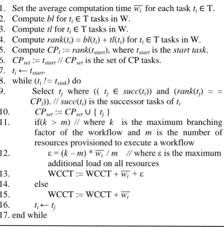
Algorithm 1. A new makespan estimation model for WCCT of the workflow
Input: A workflow W = < T, E, wi, di,j>, T and E are a set of tasks and edges in the workflow. w i , is the average computation time of the task ti and di,j is the dataflow time between the tasks ti and tj.
Output: The WCCT of the workflow.
1. Set the average computation time w i for each task ti∈ T. 2. Compute bl for ti∈ T tasks in W.
3. Compute tl for ti ∈ T tasks in W.
4. Compute rank(ti) = bl(ti) + tl(ti) for ti ∈ T tasks in W. 5. Compute CPl := rank(tstart), where tstart is the start task. 6. CPset := tstart // CPset is the set of CP tasks.
7. ti ← tstart.
8. while (ti != tsink) do
9. Select tj where (( tj ∈ succ(ti)) and (rank(tj) = =
CPl)). // succ(ti) is the successor tasks of ti 10. CPset := CPset ∪ { tj }
11. if(k > m) // where k is the maximum branching factor of the workflow and m is the number of resources provisioned to execute a workflow
12. ε = (k – m) * w i / m // where ε is the maximum additional load on all resources
13. WCCT := WCCT + w i + ε
14. else
15. WCCT := WCCT + w i 16. ti ← tj
17.end while
Fig 3: Algorithm for estimating WCCT of the workflow
Algorithm 2. A new makespan estimation model for BCCT of the workflow
Input: A workflow W = < T, E, wi, di,j>, T and E are a set of tasks and edges in the workflow. wi is the minimum computation time of the task ti and di,j is the dataflow time between the tasks ti and tj.
Output: The BCCT of the workflow.
1. Set wi to the minimum computation time of each task ti∈ T.
2. Compute bl for ti ∈ T tasks in W. 3. Compute tl for ti ∈ T tasks in W.
4. Compute rank(ti) := bl(ti) + tl(ti) for ti∈ T tasks in W. 5. CPl := rank(tstart), where tstart is the start task. 6. CPset := tstart // CPset is the set of CP tasks. 7. ti ← tstart
8. while (ti != tsink) do
9. select tj where (( tj∈succ(ti)) and ( rank(tj) = = CPl )) // succ(ti) is the successor of ti
10. CPset := CPset∪ {tj}
[image:5.595.317.543.222.451.2]11. BCCT := BCCT+ wj 12.end while.
23
5.1
Time Complexity Analysis
The computation of the WCCT of the workflow includes CP length, i.e., CPl and ε. The CP includes n1 < n tasks and e1<e edges and hence CPl can be calculated in time O(n+e) while the computation of ε involves n1 <n tasks and requires O(n) time. Therefore, the complexity of WCCT of the workflow is O(n + e), where n is the number of tasks and e is the number of edges in the workflow. The computation of BCCT of the workflow entails CPc. The calculation of CPc necessities n1 < n tasks and hence BCCT of a workflow can be computed in time O(n). Generally, the WCCT and BCCT of the workflow are computed recursively adding one task in each iteration.
The WCCT and BCCT values computed for the example workflow depicted in the Figure 1 are 508 and 195 respectively. The makespan for the same workflow generated by the HEFT [2], PETS [7] and MSL[3] scheduling strategies are 446, 446 383-time units respectively.
6.
PERFORMANCE
EVALUATION
In this section, the performance of the new makespan estimation model is evaluated using randomly generated scientific workflows namely LIGO, Epigenomics, Cybershake, and Montage. Generally, the characteristics required for generating the scientific workflows are as follows.
Workflow size (n) is the number of tasks in the workflow.
Dataflow to Computation time Ratio (DCR) is the ratio of the average dataflow time to average computation time in a workflow. The dataflow time in a workflow is computed using (11).
dataflow time = DCR * computation time
(11)
when DCR ≤ 1, computation - intensive workflows can be generated while DCR ≥ 1 workflows are data-intensive workflows. Shape parameter (α) determines the structure, i.e., the height and width of the workflow. The height of the workflow, i.e., the number of levels in a workflow is obtained by 𝑛 / α and the width of the workflow, i.e., the number of tasks at each level is 𝑛 × α. For α < 1values, longer workflows with low parallelism are generated and when α > 1, shorter workflows with high parallelism can be generated.
Heterogeneity factor (β) determines the variation in the computation times of each the task on m resources. Higher β values cause much deviation in the computation times of the tasks while lesser β values results in the trivial difference in the computation times of the tasks. The computation time of each task ti on the resource rj is denoted as wi,j, where 1 ≤ i ≤
n, 1 ≤ j ≤ m, is randomly selected from the range computed using the equation (12)
w i × (1- β / 2) ≤ wi,j ≤ w × i (1+ β / 2) (12) where w i is the average computation time of each task in
the workflow.
To evaluate the effectiveness of the new makespan estimation model, two sets of randomly generated scientific workflows are used. The first set consists of computation-intensive workflows viz., LIGO and Epigenomics workflows which are generated with workflow size (n) of {40, 56, 72, 88} and {20, 32, 64, 106} respectively.
As these workflows are computation-intensive applications, their DCR values cannot be more than one. Since the structure
of the scientific workflows is known, the parameters such as workflow size (n), DCR, heterogeneity factor (β) and average computation time of the workflow (w i ) are essential for generating the scientific workflows. The characteristics of LIGO and Epigenomics workflow set for the experimentations are depicted in Table 2.
Another set of data-intensive workflows namely Cybershake and Montage with workflow sizes (n) {20, 36, 68, 132} and {20, 38, 59, 98} respectively, are generated. Since these workflows are data-intensive applications, their DCR values cannot be less than one and the parameters are specified in Table 3. The combination of the mentioned parameter values generated 2000 workflows for each scientific workflow. The proposed BCCT and WCCTvalues for varied resource set are computed for LIGO, Epigenomics, Cybershake and Montage workflows. The BCCT and WCCT are evaluated by considering the best and the worst of the three makespans generated by the HEFT, PETS, and MSL scheduling algorithms.
Table 2. Characteristics of LIGO and Epigenomics workflows
Parameter Values
DCR 0.1 0.25 0.5 0.75 1.0
β 0.1 0.25 0.5 0.75 1
wi
100 150 200 250
m 4 8 12 16 20
Table 3. Characteristics of Cybershake and Montage workflows
Parameter Values
DCR 0.1 0.25 0.5 0.75 1.0
β 0.1 0.25 0.5 0.75 1
wi
100 150 200 250
m 4 8 12 16 20
The experimental results are presented in Table 4, 5, 6, and 7 respectively. Each row in these tables represents the average data from 20 workflows obtained with the combination of different βand w i values for each DCR value.
The validation of the new makespan estimation model is performed by comparing BCCT and WCCT values computed for each workflow with the actual makespan of the workflow. The error ξ between WCCT and the actual makespan is denoted as makespanactual and computed using (13)
actual actual makespan
WCCT makespan
13
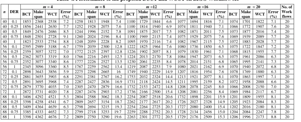
From the Table.4, it can be observed that for the computation-intensive LIGO workflows the error percent increased as DER value increased when the workflow size and the number of resources are same. Moreover, error enhanced as the workflow size increased for the same number of resources (m) and DER values. The error in percent for the workflow size 40 is noted to be 7.65, for 56 tasks it is 8.53, for 72 tasks it is 10.64 and for 88 tasks the error 13.93 percent. An error is observed to be below 10 percent for 70 percent of the cases and overall it is 10.18 percent.
24 {7.0,16.6,14.8,8.1,6.8}, and for workflow size 88 it is
{6.6,19.1, 20.4,15.3,8.3} respectively. For the same workflow size, the error is observed to vary for different number of resources. The error percent is noted to be high when the workflows attain optimal makespan. This implies that optimal schedules are attained when the number of resources provisioned are sufficient to execute the workflow.
Similar trends in the error values can also be observed for the computation-intensive Epigenomics workflow shown in Table 5. The error values are observed to be increasing with the rise
in the DER values. The error percent for workflow size {20, 32, 64, 106} is {10.89,11.33,8.81,10.61} respectively. For various m values i.e., {4, 8,12,16 20}, the error percent for workflow size 20 is {9.4,10.9,11.5,11.3,11.4}, for workflow size 32 it is {8.94,10.5,12.4,12.6,12.2}, for workflow size 64
it is {4.5,10.5, 8.8,9.8,10.4} and for 106 tasks it is {1.7,12.6, 16.1,13.3,9.3} respectively. Overall, the error value is noted to be 10.41.
For a data-intensive Cybershake workflow presented in the Table 6, the error in percent for 20 tasks is 13.64, for 36 tasks it is 13.92, for 68 tasks it is 29.6 and for 106 tasks it is 47.2. An overall error is noted to be 26 percent. For various m
[image:7.595.47.559.251.459.2]values {4, 8, 12, 16, 20}, the error in percent for workflow size 20 is {17.5, 12.4, 12.8, 12.8,12.7}, for workflow size 36 it is {17.7,18.8, 14.5,9.4,9.2}, for 68 tasks it is {21.8,33.1,34.1,31.2,26.6}and for 132 tasks it is {22.3,43.4,53.5,58.0,58.9} respectively.
[image:7.595.47.553.476.684.2]Table 4. Performance of the proposed BCCT and WCCT on LIGO Workflow set
Table 5. Performance of the proposed BCCT and WCCT on Epigenomics Workflow set n DER
m = 4 m = 8 m =12 m =16 m = 20 No. of
Work flows BCT Make
span WCT Error
(%) BCT Make
span WCT Error
(%) BCT Make
span WCT Error
(%) BCT Make
span WCT Error
(%) BCT Make
span WCT Error
(%)
40 0.1 1853 2368 2538 7.2 1258 1813 1948 7.4 1100 1729 1844 6.6 1077 1694 1816 7.1 1074 1701 1822 7.1 20 40 0.25 1856 2441 2630 7.7 1252 1928 2075 7.6 1100 1814 1940 6.9 1074 1811 1940 7.1 1066 1772 1907 7.6 20 40 0.5 1849 2476 2686 8.5 1244 1996 2152 7.8 1091 1875 2017 7.5 1082 1871 2011 7.5 1073 1877 2016 7.4 20 40 0.75 1848 2501 2728 9.1 1260 2024 2196 8.4 1100 1969 2115 7.4 1075 1929 2075 7.6 1069 1939 2089 7.7 20 40 1 1823 2533 2754 8.8 1248 2059 2228 8.2 1095 1970 2116 7.4 1082 1967 2115 7.5 1072 1883 2028 7.7 20 56 0.1 2395 2989 3188 6.7 1759 2039 2300 12.8 1222 1825 1964 7.6 1080 1736 1850 6.5 1075 1722 1847 7.2 20 56 0.25 2359 3057 3272 7.0 1772 2125 2397 12.8 1226 1902 2057 8.1 1079 1830 1961 7.1 1068 1815 1955 7.7 20 56 0.5 2362 3073 3319 8.0 1766 2216 2493 12.5 1224 2013 2170 7.8 1084 1947 2073 6.5 1075 1961 2086 6.3 20 56 0.75 2352 3077 3340 8.6 1777 2226 2527 13.5 1230 2061 2235 8.4 1078 2014 2151 6.8 1065 1995 2141 7.3 20 56 1 2345 3096 3360 8.5 1767 2259 2562 13.4 1219 2087 2253 7.9 1080 2021 2162 6.9 1070 1940 2072 6.8 20 72 0.1 2898 3643 3856 5.9 2275 2298 2665 16 1749 1940 2229 14.9 1207 1816 1954 7.6 1078 1769 1880 6.3 20 72 0.25 2881 3655 3903 6.8 2291 2381 2767 16.2 1753 2032 2324 14.4 1213 1921 2077 8.1 1070 1863 1997 7.1 20 72 0.5 2891 3695 3968 7.4 2287 2427 2836 16.9 1731 2118 2424 14.5 1211 1995 2159 8.2 1072 1958 2088 6.6 20 72 0.75 2879 3770 4035 7.0 2305 2470 2879 16.6 1732 2153 2472 14.8 1208 2078 2245 8.0 1066 2008 2150 7.0 20 72 1 2872 3731 4020 7.8 2287 2476 2903 17.2 1736 2166 2500 15.4 1208 2081 2256 8.4 1069 1984 2117 6.7 20 88 0.1 3406 4292 4521 5.3 2804 2588 3062 18.3 2254 2087 2518 20.6 1732 1898 2201 15.9 1201 1809 1955 8.1 20 88 0.25 3398 4258 4541 6.7 2809 2657 3154 18.7 2262 2177 2617 20.2 1726 2027 2328 14.9 1205 1923 2084 8.3 20 88 0.5 3409 4364 4639 6.3 2798 2694 3215 19.3 2254 2264 2725 20.3 1727 2080 2400 15.4 1202 2016 2180 8.1 20 88 0.75 3385 4333 4652 7.3 2799 2718 3253 19.7 2259 2288 2752 20.3 1728 2134 2456 15.0 1204 2084 2247 7.8 20 88 1 3398 4362 4676 7.2 2809 2750 3290 19.6 2263 2301 2772 20.5 1729 2176 2509 15.3 1206 1996 2173 8.8 20
n DER
m = 4 m = 8 m =12 m =16 m = 20 No. of
Work flows BCT Make
span WCT Error
(%) BCT Make span WCT
Error (%) BCT
Make span WCT
Error (%) BCT
Make span WCT
Error (%) BCT
Make span WCT
Error (%)
25
Table 6. Performance of the proposed BCCT and WCCT on Cybershake Workflow set
Table 7. Performance of the proposed BCCT and WCCT on Montage Workflow set
For Montage workflow depicted in the Table 7, for lower workflow sizes the error percent is high and as the workflow size increased the error is observed to decline. It can be observed that error increased with DER values. The error for the workflow size 20 is observed to be 39.72 percent, it is 27.82 percent for 38 tasks, 17.98 percent for 59 tasks, and increased to 28 percent for 98 tasks. And overall error is 28 percent.
7.
CONCLUSION
A new makespan estimation model is devised to estimate the bounds on the makespan of the workflows. In the available model’s dataflows were either ignored or nominal, hence these models could not be extended for computation-intensive and data-intensive workflows. The proposed makespan estimation model is devised with minimal information considering the profile of the workflow as the makespan of the workflow highly depends on its profile. The proposed estimation model is devised with a complexity of O(n) and O(n+e) for computing BCCT and WCCT respectively. The present model is validated using the scientific workflows. The results of the experiments revealed that the proposed model could precisely estimate the makespan of the scientific workflows. The error for computation-intensive workflows
namely LIGO and Epigenomics is observed to be 10.18 and 10.4 percent respectively and for data-intensive workflows namely Cybershake and Montage it is noted to be 26 percent and 28 percent respectively.
8.
REFERENCES
[1] M.R., and D.S.Johnson, “Computers and intractability: A guide to the theory of NP-completeness,” W.H.Freeman and Co., San Franisco, CA, 1979.
[2] H.Topcuoglu, S.Hariri, and M.Y.Wu, “Performance effective and low-complexity task scheduling for heterogeneous computing,” IEEE Trans. Parallel Distributed Systems,vol.13 (3), pp.260–274, 2002.
[3] D.Sirisha, and G.Vijayakumari, “Minimal start time heuristics for scheduling workflows in heterogeneous processing systems, ” Distributed Computing and Internet Technology, Springer Lecture Notes in Computer Science, vol.9581, pp.199-212, 2016.
[4] E.B.Fernandez, and B.Bussell, “Bounds on the number of resources and time for multiresource optimal schedules,” IEEE Trans. Computers, vol.22(8), pp.745-751,1973.
n DER
m = 4 m = 8 m =12 m =16 m = 20 No. of
Work flows BCT Make
span WCT Error
(%) BCT Make span WCT
Error (%) BCT
Make span WCT
Error (%) BCT
Make span WCT
Error (%) BCT
Make span WCT
Error (%)
20 1 173 292 342 17.0 165 274 300 9.6 162 269 296 10.2 160 269 297 10.4 158 270 297 10.0 20
20 2 171 374 436 16.4 165 357 392 10.0 162 358 394 10.0 160 357 394 10.2 161 354 392 10.8 20
20 5 172 604 704 16.6 166 601 671 11.7 162 575 651 13.1 160 593 665 12.2 160 607 677 11.5 20
20 7 173 729 859 17.9 166 723 824 14.0 163 728 830 13.9 161 711 814 14.5 159 718 821 14.4 20
20 10 172 896 1072 19.7 164 892 1041 16.7 163 894 1043 16.8 160 904 1053 16.6 160 765 894 16.8 20
36 1 177 439 516 17.6 166 316 390 23.5 164 284 337 18.8 160 285 310 8.7 160 278 303 9.0 20
36 2 174 512 603 17.8 170 404 488 20.9 165 387 447 15.6 160 384 417 8.4 159 385 417 8.5 20
36 5 181 731 862 17.9 168 653 771 18.1 164 662 750 13.2 160 642 705 9.9 159 646 709 9.7 20
36 7 174 858 1017 18.6 165 829 966 16.5 162 812 925 13.9 160 813 896 10.2 159 822 903 9.9 20
36 10 178 1133 1321 16.6 169 1103 1266 14.8 163 1144 1273 11.3 160 1122 1229 9.5 160 960 1047 9.1 20
68 1 177 657 782 22.4 166 396 541 43.1 164 325 459 48.4 160 294 409 45.9 160 286 379 38.4 20
68 2 174 739 873 21.4 170 483 638 37.6 165 415 556 40.1 160 389 511 37.0 159 382 482 30.8 20
68 5 181 929 1102 21.9 168 710 896 30.8 164 655 827 30.7 160 642 792 27.5 159 635 761 23.4 20
68 7 174 1068 1264 21.6 165 848 1057 29.0 162 814 1005 27.6 160 806 975 24.7 159 806 949 20.8 20 68 10 178 1255 1489 21.9 169 1105 1340 25.1 163 1078 1293 23.5 160 1076 1270 21.2 160 926 1078 19.4 20
132 1 148 1171 1439 22.9 139 653 997 52.7 135 481 831 72.6 133 398 737 85.3 132 361 679 88.1 20
132 2 145 1266 1543 21.9 139 734 1090 48.5 135 568 929 63.6 134 492 840 70.6 133 453 779 72.1 20 132 5 149 1458 1780 22.1 141 941 1337 42.0 138 797 1196 50.0 135 734 1116 52.1 134 714 1072 50.1 20 132 7 147 1580 1931 22.2 136 1088 1511 38.9 138 962 1382 43.7 133 902 1304 44.7 132 882 1264 43.3 20 132 10 146 1780 2178 22.3 137 1323 1782 34.7 136 1208 1661 37.5 133 1165 1599 37.2 133 966 1361 41.0 20
n DER
m = 4 m = 8 m =12 m =16 m = 20 No. of
Work flows BCT Make
span WCT Error
(%) BCT Make span WCT
Error (%) BCT
Make span WCT
Error (%) BCT
Make span WCT
Error (%) BCT
Make span WCT
Error (%)
20 1 322 474 537 13.2 303 468 531 13.3 299 480 537 11.9 295 465 527 13.3 292 459 525 14.3 20
20 2 327 624 718 15.2 308 618 721 16.6 298 609 712 16.8 295 607 712 17.4 292 612 715 16.9 20
20 5 323 817 996 29.2 307 856 1024 32.8 299 857 1023 32.2 295 850 1016 32.4 293 852 1018 32.4 20 20 7 327 870 1142 41.7 304 882 1139 48.4 298 873 1130 48.9 296 892 1143 47.1 295 905 1156 46.4 20 20 10 319 720 1005 79.0 307 726 1007 96.5 300 727 1005 95.8 296 721 1000 96.8 293 673 900 84.5 20
38 1 327 628 714 13.8 310 554 643 16.2 299 548 605 10.3 293 537 595 10.8 293 533 594 11.4 20
38 2 327 779 922 18.4 302 751 894 19.1 298 754 863 14.5 295 747 861 15.3 292 741 853 15.1 20
38 5 320 1135 1459 28.6 303 1138 1431 32.3 299 1156 1410 27.5 294 1139 1409 29.6 293 1129 1400 30.0 20 38 7 322 1370 1822 33.0 301 1374 1781 37.1 301 1377 1765 35.2 295 1328 1746 39.3 293 1367 1757 35.6 20 38 10 320 1640 2218 39.2 303 1619 2185 48.6 298 1629 2165 45.7 294 1645 2171 44.3 294 1388 1829 44.1 20
59 1 324 774 871 12.5 306 582 715 23.0 300 551 657 19.3 299 545 616 13.0 294 541 588 8.8 20
59 2 325 909 1041 14.5 301 736 909 23.5 296 718 860 19.8 298 722 829 14.9 298 716 798 11.5 20
59 5 335 1302 1540 18.2 306 1225 1508 23.1 299 1219 1468 20.4 295 1216 1431 17.7 292 1225 1414 15.5 20 59 7 325 1621 1920 18.5 309 1560 1915 22.7 300 1558 1877 20.5 301 1558 1845 18.5 292 1558 1817 16.6 20 59 10 331 2095 2481 18.4 304 2072 2531 22.1 300 2066 2492 20.6 297 2069 2462 19.0 297 1749 2049 17.1 20
98 1 319 1097 1234 12.5 307 734 961 30.9 298 633 847 33.8 295 597 787 32.0 291 584 741 26.9 20
26 [5] K. Jain Kumar, and V. Rajaraman, “Lower and upper
bounds on time for multiresource optimal schedules,” IEEE Transactions on Parallel and Distributed Systems, vol.5(8), pp.879-886,1994.
[6] S. Bharathi, A. Chervenak, E. Deelman, G. Mehta, M.-H. Su, and K. Vahi, “Characterization of scientific workflows,” 3rd
Workshop on Workflows in Support of Large-Scale Science, pp.1-10, Nov. 2008.
[7] E.Illavarasan, and P.Thambidurai, “Low complexity performance effective task scheduling algorithm for heterogeneous computing environments,” Journal of Computer Science, vol.3(2), pp.94-103, 2007.
[8] I. Pietri, G. Juve, E. Deelman and R. Sakellariou, "A Performance model to estimate execution time of scientific workflows on the cloud,” 9th Workshop on Workflows in Support of Large-Scale Science, New Orleans, LA, pp. 11-19, 2014.
[9] Berriman G, Laity A, Good J, Jacob J, Katz D, Deelman E, Singh G, Su M, Prince T., “Montage: The architecture and scientific applications of a national virtual observatory service for computing astronomical image mosaics,” Proceedings of Earth Sciences Technology Conference, 2006.
[10] Graves R, Jordan TH, Callaghan S, Deelman E, Field E, Juve G, Kesselman C, Maechling P, Mehta G, Milner K, “Cybershake: A physics-based seismic hazard model for southern california,” Pure and Applied Geophysics, vol. 168(3-4), pp.367–381,2011.
[11] Abramovici A, Althouse WE, Drever RW, G¨ursel Y, Kawamura S, Raab FJ, Shoemaker D, Sievers L, Spero RE, Thorne KS, “Ligo: The laser interferometer gravitational-wave observatory Science,” vol. 256 (5055), pp.325–333,1992.
[12] USC Epigenome Center. http :// epigenome.usc.edu. Accessed : October 2015.