Pre Decision Side Bet Sequences

Pre-Decision Side-Bet Sequences

Kim Kaivanto and David Peel

Department of Economics, Lancaster University, Lancaster LA1 4YX, UK

this version:

March 2019

Abstract

Risk-averse Expected Utility (EU) decision makers with wealth-dependent utility

func-tions may find themselves indifferent between accepting and rejecting an indivisible risky

prospect. Bell (1988) showed that under these circumstances it may be EU-enhancing for

the decision maker to engage in an actuarially fair pre-decision side bet, accepting the

indivisible risky prospect conditional upon winning the side bet. In this letter we show

that decision makers restricted to actuariallyunfair side bets may optimally engage in a

sequence of individually EU-enhancing side bets. This contrasts with the case of

actuari-ally fair side bets where only one such bet will be undertaken. The actuariactuari-ally unfair side

bet’s optimal stake size can be a significant proportion of the individual’s initial wealth.

Nevertheless after losing the side bet wealth may still remain within the interval of interim

(utility) convexity, whereupon it is optimal to place another side bet.

Keywords: Expected Utility, risk aversion, side bets, rationality, indivisibility,

discrete-ness, actuarial fairness

JEL classification: D81

1 Introduction

Bell (1988) showed that for decision makers with wealth-dependent utility functions local convexity can emerge on an interim basis for globally risk-averse decision makers who are in possession of a standing offer to acquire a discrete, indivisible risky prospect. Global risk aversion notwithstanding, then, a normatively rational EU decision maker can benefit by increasing her risk exposure through a pre-decision side bet when within such a region of interim local convexity. This seemingly counterintuitive result applies in the neighborhood of any wealth level at which a risky prospect switches from being EU-diminishing to being EU-augmenting. Bell only considered an actuarially fair side bet and demonstrated that only one such bet will be undertaken. However we demonstrate in this letter that if the individual is restricted to actuarially unfair side bets, in the event of losing an actuarially unfair side bet, the decision-maker’s wealth is diminished, but not necessarily by enough to fall out of the interval of interim convexity. Hence, a second optimally EU-enhancing side bet may be constructed, the stake of which is smaller than that of the first side bet, keeping the decision maker within the interval of interim convexity. When the decision maker is indifferent between her initial certain wealth and acquiring the indivisible risky prospect, not only will it be possible to construct a single actuarially unfair optimal side bet, but in general a sequence of individually optimal actuarially unfair side bets may be constructed, given continual availability of the side bets at ever-longer odds.

2 Single side bet

We follow Bell (1988) in illustrating the single-side-bet case with a logarithmic-utility ex-ample in which the decision maker’s initial wealth isw0 =£10,000. The decision maker is

in possession of a standing offer to acquire the risky prospectg0 = (£10,000,1₂; −£5000,1₂).

We write the prospect in net-final-wealth terms as g(g0, w0) = (£20,000,1₂; £5,000,1₂).

Define this to be the round-zero lottery L0 =g(g0, w0). Since

E[u(L0)] = 1₂ln(£20,000) +1₂ln(£5,000) = ln(£10,000) =u(w0) (1)

the decision maker is indifferent between acquiring the risky prospect and sticking with her initial (certain) wealth.

Now let the decision maker consider a pre-decision side betg1 = (£1,000,₂1;−£1,000,1₂).

Although g1 and g0 are stochastically independent, the decision maker considers a

com-pound, conditional policy of only acquiring the round-zero lotteryL0 if the side bet proves

successful. This compound lottery, which presumes the Reduction of Compound Lotteries (ROCL) axiom, may be written as follows.

L1(g(g0, w0), g1) = £21,000,₄1; £6,000,1₄; £9,000,1₂

(2)

Although the side bet g1 is EU-diminishing in isolation due to risk aversion, when g0 is

implemented conditional upon successful resolution ofg1, the resulting compound lottery

is EU-augmenting.

The Certainty Equivalent (CE) of this compound lottery is £10,002.1 _{This is a marginal}

(£2) improvement, reflecting the arbitrary nature of the side bet g1. By appropriate

choice of the side bet, it will in principle be possible to improve upon this CE.

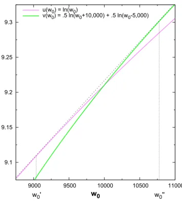
An EU-augmenting side bet can be constructed only if the decision maker’s wealth falls within the interval of interim convexity. The bounds of this interval also determine the payoffs and probabilities of the optimal side bet. Figure 1 illustrates the decision-maker’s utility functionu(·) without the risky prospect andv(·) with the risky prospect. The com-mon tangent tou(·) andv(·) identifies the lower and upper bounds of the interval of interim convexity (w₀0, w00₀). The solution method for identifying these bounds analytically is pre-sented in Appendix A. This yields the numerical values (w₀0, w00₀) = (9037.16,10774.6). Given the decision-maker’s assumed wealth in this example, an EU-augmenting side bet is possible since 10,000 ∈ (9037.16,10774.6), and the unconstrained optimal side bet is given byg₁∗ = (w00₀−w0,

w0−w00

w00₀−w0₀; w

0

0−w0,

w00

0−w0

w₀00−w0₀) = (£774.6,0.554; −£962.84,0.446). With

this optimal pre-decision side bet g∗₁, the compound lottery becomes

L1(g(g0, w0), g1∗) = (£20774.6,0.277; £5774.6,0.277; £9037.16,0.446) (4)

and the decision maker increases her utility

E[u(L1(g(g0, w0), g1∗))] > E[u(L1(g(g0, w0), g1))] > u(w0) (5)

to the CE wealth level of £10,052.8, which is clearly greater than the £10,002 of the arbitrary side bet g0.

3 Sequence of actuarially unfair side bets

We now demonstrate the new result that a sequence of side bets may be optimal. Here we focus on actuarially unfair ‘wager’ side bets based on European Roulette. The (negative) expected return per unit staked at European Roulette is µ = −1

37. Odds are denoted

a. For a single-number bet in European roulette, the payout odds are 35:1, that is a = 35₁. The associated win probability is p = 1+₁₊µ_a, which for the single-number bet is p= (1 + −₃₇1)/(1 + 35₁) = ₃₇1 . Here for illustrative purposes and to illustrate the length of the betting sequence we assume that odds are offered at all probabilities with a negative expected rate of return of −1

37. Meanwhile, the interim-convexity bounds remain as

above.2 _{To determine the optimal round-one counterparty-constrained optimal side bet,}

we maximize

p

1

2ln(w0+ 10,000 +sa) + 1

2ln(w0−5,000 +sa)

+ (1−p) ln(w0−s)−ln(w0) (6)

by appropriate choice of stakesand payout oddsa. As the win probabilitypis a function ofaand the fixed parameterµ, there are no other undetermined parameters. This is solved by settings = 573.33 andsa = 732.77 – i.e. smaller than in the unconstrained, actuarially fair problem – from which follows that a = 732.77/573.33 = 1.27809 and consequently p = (1 −(1/37))/(1 + 1.27809) = 0.42710. Due to the house advantage µ = −₃₇1, the expected value of this side bet is |µ|s = £15.50 less than in the unconstrained problem,

1_E[u(L

1)] =u(£10,002)

Figure 1: Common tangent to u(·) and v(·) which determines the bounds of the interval of interim convexity (w₀0, w00₀) for the round-one side bet.

9.1 9.15 9.2 9.25 9.3

9000 9500 10000 10500 11000

w

w

'

w

''

u(w₀) = ln(w₀)

v(w₀) = .5 ln(w₀+10,000) + .5 ln(w₀-5,000)

i.e. E[w0+psa−(1−p)s] =£10,000−£15.50 =£9,984.50.

L1(g(g0, w0), g∗1|µ) = (£20732.77,0.21355; £5732.77,0.21355; £9,426.67,0.5729) (7)

With the optimal counterparty-constrained pre-decision side bet g∗₁|µ, the CE of this

compound lottery (7) becomes £10,030.69, in which the £30.69 increase over the pre-side-bet CE is 58% of the £52.80 increase achieved with the actuarially fair side bet g₁∗. Still, with the counterparty-constrained optimal side bet g₁∗|µ the compound lottery

L1(g(g0, w0), g1∗|µ) nevertheless proves to be EU-augmenting.

E[u(L1(g(g0, w0), g∗1))] > E[u(L1(g(g0, w0), g1∗|µ))] > E[u(L1(g(g0, w0), g1))] > u(w0)

4 Sequences of individually optimal side bets

When side bets are constrained to be actuarially unfair, the round-one side-bet stake is smaller than the difference between initial wealth w0 and the lower bound of the interval

of convexityw0₀. Hence, after losing the side bet g₁∗|µ in the round-one compound lottery

L1(g(g0, w0), g1∗|µ) and therefore the associated stakes∗1µ=£573.33, the decision-maker’s

wealth is reduced to w1 =£9,426.67∈(w00, w000), which is within the interval of convexity.

Consequently the decision-maker can benefit from a further side-bet round. In turn the stake of the optimal round-two side bet s∗_2µ=£135.25 is also smaller thanw1−w00. Upon

losing the side bet of the round-two compound lottery L2(g(g0, w1), g2∗|µ), the

decision-maker’s wealth is reduced to w2 =£9,291.43∈ (w00, w

00

0), which is within the interval of

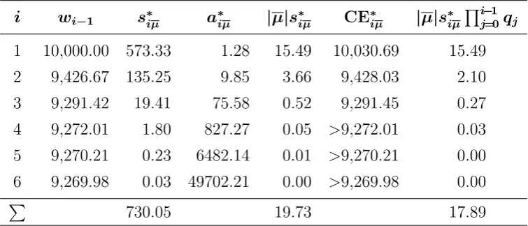
convexity. Again the decision maker can benefit from a further side-bet round. Table 1 presents this sequence of individually EU-augmenting optimal side bets. These side bets have been computed under the assumption that the minimum stake-size increment is 0.01 (one penny). The round-four side bet’s CE∗_4µis larger thanw3 in the fourth decimal digit.

Similarly CE∗_5µ > w4 in the sixth decimal digit, and CE∗6µ > w5 in the eighth decimal

digit. Notice that availability of ever-longer-odds side bets is necessary for extending the sequence, which nevertheless is truncated to six rounds due to the discrete, one-penny stake-size increment.

Table 1: Parameters of optimal EU-augmenting round-i side bets in European roulette (µ= −₃₇1).

i wi−1 s∗_iµ a_iµ∗ |µ|s∗_iµ CE∗_iµ |µ|s∗_iµ Qi−1

j=0qj

1 10,000.00 573.33 1.28 15.49 10,030.69 15.49

2 9,426.67 135.25 9.85 3.66 9,428.03 2.10

3 9,291.42 19.41 75.58 0.52 9,291.45 0.27

4 9,272.01 1.80 827.27 0.05 >9,272.01 0.03

5 9,270.21 0.23 6482.14 0.01 >9,270.21 0.00

6 9,269.98 0.03 49702.21 0.00 >9,269.98 0.00

P

730.05 19.73 17.89

4.1 Maximally unfair case

Here we ask, what is the mostdisadvantageous per-unit-bet expected return µ

¯ that the decision maker will still find EU enhancing?

Two of the parameters determining µ

¯ may be treated as exogenous for present pur-poses. The first captures the decision maker’s ‘just-noticeable difference’, operationalized as the number of significant digits to which EU and are measured. The second captures the house minimum-stake-size increment (here assumed to be 1 penny). Operationally we maximize |µ

¯| subject to (i) the discrete 1-penny minimum-stake-size increment and (ii) the requirement that the round-i side bet be EU-enhancing (wi−1 −CE∗iµ

¯

Table 2: Parameters of individually optimal EU-augmenting round-i side bets for maxi-mally disadvantageous, but still EU-augmenting mean return (µ

¯=−0.19).

i wi−1 s∗_iµ

¯

a∗_iµ

¯ |µ ¯|s ∗ iµ ¯

CE∗_iµ

¯ |µ ¯|s ∗ iµ ¯

Qi−1

j=0qj

1 10,000.00 1.11 45.338 0.21 >10,000.00 0.21

2 9,998.89 0.90 75.998 0.17 >9,998.89 0.17

3 9,997.99 0.16 564.422 0.03 >9,997.99 0.03

4 9,997.83 0.07 1146.683 0.01 >9,997.83 0.01

P

2.24 0.42 0.42

any arbitrarily fine-grained just-noticeable difference. Table 2 presents the sequence of individually EU-enhancing side bets which follows the first-round stake and mean-return combination (s∗_1µ

¯

, µ

¯) = (1.11,−0.19).

5 A tie-breaking rule?

Since the side-bet strategy breaks the decision maker’s indifference between initial wealth w0 and the indivisible risky prospect L0, it is natural to query the extent to which the

side-bet strategy can be understood as atie-breaking rule. And if this conception is valid, what function can a side bet perform once the first side-bet is played out, and wealth deviates from the indifference level w0?3

This is an incisive question that demands careful revisitation of the tie-breaking litera-ture. A tie-breaking rule may be understood “as a second strict and transitive preference relation that the agent consults only when he is indifferent” (Kimya 2017, p. 140). Cru-cially, however, a tie-breaking rule does not alter the decision maker’s underlying prefer-ence ordering. The indifferprefer-ence class remains unchanged by the tie-breaking rule, as does the rest of the preference ordering above and below the indifference class.

Meanwhile, Bell’s (1988) side-bet strategy constitutes a new ‘act’ – a non-redundant mapping from the set of states to the set of consequences – which increases the decision maker’s utility above that delivered by initial wealth alone or by directly undertaking the indivisible round-zero lotteryL0. As a new act, it alters the set of available non-redundant

choice options, and thus it also alters the decision maker’s underlying preference ordering. Hence, Bell’s (1988) side-bet strategy is not a ‘tie-breaking rule’ in a formal sense as it is understood in the literature.

A careful reading of Bell (1988) shows that the side-bet strategy differs from a tie-breaking rule in a second sense: “This strategy works in the neighborhood of any wealth level at which alternative switches from being unattractive to being attractive” (emphasis added, p. 797). The side-bet strategy offers the prospect of enhanced expected utility when wealth is in the non-degenerate interval of interim convexity.

The possibility for side-bet sequences arises precisely because the decision maker’s optimal side-bet’s stake is smaller when wagering opportunities are unfair (µ < 0), and therefore even if she loses the side bet, she remainswithin the interval of interim convexity.

6 Conclusion

In this note we revisit Bell’s (1988) finding that a pre-decision side bet can be a ratio-nal, EU-enhancing strategy for determining whether to take on a large, indivisible, risky prospect. When pre-decision side bets are constrained to be actuarially unfair, unlike in Bell’s presentation, the side bet’s optimal stake size is biased downward. Upon los-ing the side bet, the decision maker’s wealth consequently remains within the interval of interim convexity, instead of being ejected to its lower boundary. Hence, the decision maker rationally engages in a further side-bet round. Under the assumptions of Bell’s (1988) example, we find that the decision maker rationally engages in up to four side-bet rounds (in one case, six rounds). For each successive optimal side bet, the stake becomes smaller and the required odds become longer. This ever-longer-odds requirement may hinder implementation of extended side-bet sequences in practice. Nevertheless side-bet sequences are surprisingly general from a theoretical standpoint, as they arise in all fam-ilies of non-linear, non-exponential risk-averse utility functions.4 _{Together with Bell’s}

(1988) seminal result, the present finding expands the range of empirical phenomena that can be explained within the framework of normative rationality. However, it also intro-duces a further set of methodological considerations that must be confronted in the design of risk-aversion-elicitation procedures and in the empirical estimation of risk-aversion co-efficients.

References

Bell, D. E. (1988) “The value of pre-decision side bets for utility maximizers”Management

Science 34(6), 797–800.

Kimya, M. (2017) “Nash implementation and tie-breaking rules” Games and Economic

Behavior 102, 138–146.

Quiggin, J. (1993) Generalized Expected Utility Theory: The Rank-Dependent Model.

Kluwer Academic: Boston, MA.

4_{We have found that this effect may be replicated with Rank-Dependent Expected Utility (Quiggin,}

A Side-bet bounds

The tangent line to u(·) at (w0₀, u(w₀0)), where u(w0) = ln(w0), is

y = u(w0₀) +u0(w0₀)(w0−w00) (9)

= ln(w₀0) + w0−w

0

0

w₀0 (10)

while the tangent line tov(·) at (w₀00, v(w00₀)), wherev(w0) = 1₂ln(w0+ 10,000) +1₂ln(w0−

5,000), is given by

y = u(w₀00) +u0(w₀00)(w0−w000) (11)

= 1 2

ln(w₀00+ 10,000) + ln(w₀00−5,000) + w0−w

00

0

w00

0 + 10,000

+ w0−w

00

0

w00

0 −5,000

. (12)

In order for these lines to be the same (i.e. a common tangent to u(·) and v(·)) then they must share the same slope

1 w0

0

= 1

2(w00

0 + 10,000)

+ 1

2(w00

0 −5,000)

(13)

and vertical intercept

ln(w₀0)−1 = 1 2

ln(w00₀ + 10,000) + ln(w00₀ −5,000)− w 00

0

w00₀ + 10,000 −

w00₀ w₀00−5,000

.