The Dynamic Analysis of the Cash Flows on ATM

http://www.scirp.org/journal/jcc ISSN Online: 2327-5227 ISSN Print: 2327-5219

DOI: 10.4236/jcc.2018.64003 Apr. 26, 2018 38 Journal of Computer and Communications

The Dynamic Analysis of the Cash Flows on

ATM

Zhengyou Wang

Department of Film and Television Arts, Shanghai Publishing and Printing College, Shanghai, China

Abstract

Based on the time series of cash flows on ATM, the varying rule of withdrawal is analyzed. The model of autoregression and moving average is established by Matlab and the reliability is checked. According to the model, the cash flows on ATM are forecasted in the coming 10 days. It is important for banks to prepare the cash.

Keywords

Cash Flows, Autoregression Model, Dynamic Analysis, Forecast

1. Introduction

As the pace of life is accelerating, the application of ATM (Automated Teller Machine) becomes wider and wider. Every day, there is considerable amount of cash withdrew through the means of ATMs. Therefore, how to accurately pre-dict the daily ATM cash flows becomes a significant issue for banks in their preparation and allocation of cash. This article, based on the known time series of ATM cash flows, analyzes the varying rules of cash withdrawal amount of ATMs. It builds an autoregressive and moving average model (ARMA) (p, q) via model recognition and parameter estimation. Based on the model, ATM cash flows for the coming 10 days are forecasted.

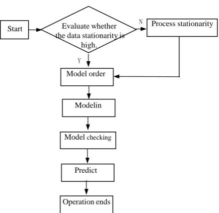
The main steps for predicting ATM cash flows by using time series analysis are as shown in Figure 1.

2. Mathematical Model

Since the observed time series data often contains random interference compo-nents, the building of mathematic model for time series will offset the interfe-rence to the maximum, so as to focus on the essential characteristics of time series.

How to cite this paper: Wang, Z.Y. (2018) The Dynamic Analysis of the Cash Flows on ATM. Journal of Computer and Com-munications, 6, 38-43.

https://doi.org/10.4236/jcc.2018.64003

Received: March 19, 2018 Accepted: April 23, 2018 Published: April 26, 2018

Copyright © 2018 by author and Scientific Research Publishing Inc. This work is licensed under the Creative Commons Attribution International License (CC BY 4.0).

http://creativecommons.org/licenses/by/4.0/

DOI: 10.4236/jcc.2018.64003 39 Journal of Computer and Communications Figure 1. ATM cash flows predicting procedures.

Time series analysis is a fast developing discipline due to its wide range of appli-cation, which leaves us enormous mathematic models illustrating time series. Main models include ARIMA (autoregressive integrated moving average mod-el), wavelet model, and neural network model [1] [2] [3]. However, this article adopts the most typical model and a model applied most widely—the autore-gressive moving average model for the illustration of the varying rules of ATM cash flows.

2.1. Data Import

Time series is featured by that the data values vary with time, which means, there is great randomness in values or locations of points for different moments. It is not possible to accurately predict values by historical values. However, the values before and after the moment or the location of data points have certain correlations [4] [5] [6]. This article adopts Matlab as the tool for modeling and analysis. It imports original data of daily withdrawal of an ATM in the year of 2016, which constitutes the time series to be analyzed and is stored in the system as output column vector

{

( )

}

2.2. Stationarity Evaluation

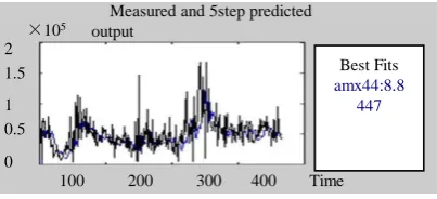
Use Matlab toolbox to analyze the stationarity of time series and employ default ARMA models and relevant parameters provided by Matlab for time series modeling. As shown in Figure 2, the stationarity of original data is weak.

By observing the fit of the model, we can find that: the fit of the model is 3.3381. Since the stationarity of the model is relatively weak, the fit of the model is not strong. Therefore, the original data requires stationarity processing.

2.3. Data Preprocessing

In order to better model and predict, data should be firstly subject to stationarity N

Start

Model order

Modelin

Model checking

Predict

Operation ends Evaluate whether the data stationarity is

high.

Y

DOI: 10.4236/jcc.2018.64003 40 Journal of Computer and Communications processing. The method adopted is to differencing the data by EXCEL and get a more stationary group of series. Import the processed data into Matlab and we will see Figure 3 in the Matlab toolbox.

The stationarity of the series curve after stationarity processing is better than the curve of original data, and the fit of the model is also better than the original ones. As shown in Figure 4, compared with the original time series, the time se-ries after preprocessing offset the trend components of the original time sese-ries, which means, the processed one filters out the low frequency part.

2.4. Order Determination

After stationarity processing, it is the stage of order determination, which means, to determine the values of p and q in ARMA (p, q). Since the order de-termination is different, the consequent fit values of models are different. Hence, the choosing of a proper order is vital for determining the fit between the model and original data and also for the accuracy of data prediction after modeling.

There are a number of methods for order determination, such as FPE, AIC, BIC and etc. Test in accordance with the following orders which are arranged from low to high orders: ARMA (2, 1) ARMA (1, 1), ARMA (3, 2), ARMA (3, 1), ARMA (2, 2), ARMA (4, 3), ARMA (4, 2), ARMA (4, 1), ARMA (3, 3) and ARMA (4, 4) models. The order is determined through the fit values between the series and models of different orders.

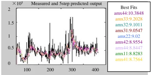
Comparison of model fit is shown in Figure 5.

Figure 2. Time series plot of original data.

Figure 3. Series after stationarity processing.

Figure 4. Comparison of model fit.

1.6

1.2

50 100 150 200 250 300 350 400 1.4

1.0 0.8 0.6 0.4 0.2 0.0 1.8 2

×105

Measured and 5step predicted output

Time 2

Best Fits amx44:8.8

447 1.5

1

0.5

0

100 200 300 400

DOI: 10.4236/jcc.2018.64003 41 Journal of Computer and Communications Figure 5. Comparison of model fit.

It is concluded that the model fit of (p = 4, q = 3) is better than the fit chart of other selected orders. Therefore, ARMA (4, 3) is selected.

And the standard form of the ARMA model is:

( )

( )

1 1

1 1

p q

i j

i j

i j

a B x t c B ε t

= =

 

 ₋  ₌ ₋ 

   

 



∑

∑

In which, B is the backward shift operator and

ε

( )

model may be simplified as:

( ) ( )

( ) ( )

A B x t =C B x t

The model after order determination is outputted as:

( )

1 2.444 2.07 0.6207

C B = − B+ B − B

( )

1 2.444 2.07 0.6207

C B = − B+ B − B

2.5. Model Checking

First evaluate the independency of the model residual, that is, to evaluate wheth-er analyzing residuals have autocorrelation, so as to get the corresponding resi-dual analysis graph Figure 6.

In Figure 6, we can see clearly that the residuals are strictly distributed be-tween −0.1 and 0.1, by which we can conclude that the model residuals have no autocorrelation and the independency of the model residuals are strong. There-fore, this ARMA model is suitable for simulating this time series.

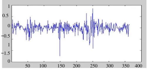
In addition, difference analysis is conducted and the residual plot is as shown in Figure 7.

Besides, by calculation, we can get the average error of 14.12% (Average accu-racy is 85.88%), which proves that this model has sound original data for fit and that this model may be employed to predict future values.

3. Predict

After the model is built, we proceed to the stage of prediction. The adopted principle for prediction is to obtain corresponding estimates through simulation of data by the model and the estimates are the predicted values. The prediction may be easily completed by using Matlab toolbox. This is the predicted cash

1.5

1

0.5

0

100 200 300 400

×105 _{Measured and 5step predicted output}

2 Best Fits

amx44:10.3848

amx33:9.2028 amx32:9.1011 amx31:9.0547

amx22:9.02

DOI: 10.4236/jcc.2018.64003 42 Journal of Computer and Communications Figure 6. Residual analysis graph.

Figure 7. Residual plot.

flows of this ATM for the next 10 days. The predicted values for the next 10 days are:

71.850, 40.116, 52.453, 56.345, 57.699, 62.215, 65.810, 52.470, 44.929, 41.179.

4. Conclusions

Data analysis is always a popular topic for research, creating various new cross-disciplines. It gathers research findings of various disciplines including machine learning, database, pattern recognition, statistics, AI, management in-formation system and etc., and attracts experts and scholars of different back-grounds to engage in research and development in this area. It is deemed as an important tool bringing huge returns by the business circles. Especially, the uti-lization of times series research methods in solution and prediction of actual is-sues are applied in a wide range of areas. It has been transferred from pure theo-retical studies to more practical connection, integration and application in the real world and engineering practices. By using the varied types of times series and through analysis and choosing of proper mathematic models, we can predict future occurrence and realize our purpose of understanding of things.

This article predicts cash flows of an ATM by analyzing the ATM cash flows data and building ARMA models. As we all know, the application of ATM is an integral part of a society of which the life pace is speeding up. Every day, there is a considerable amount of cash withdrew by means of ATMs. Therefore, the ac-curate prediction of daily cash flow is of great importance for banks and corres-ponding organizations in preparation and allocation of cash.

0.2

0.1

0

−0.2

−0.1

−20 −10 0 10 20

1 0.5

0

−0.5

−1.5 0

DOI: 10.4236/jcc.2018.64003 43 Journal of Computer and Communications

References

[1] Tian, Z. (2016) Theories and Methods for Dynamic Data Processing—Time Series Analysis. Northwest University Press, Xi’an.

[2] Chen, Z.G. (2016) Time Series and Spectrum Analysis. Science Press, Beijing. [3] Guo, G.D. (2015) Data Simplification and Categorization Based on Space Division.

Journal of Chinese Computer Systems, 23, 456-459.

[4] Ganti, V., Gehrke, J. and Ramakrishnan, R. (2013) DEMO: Mining and Monitoring Evolving Data. IEEE Transactions on Knowledge and Data Engineering, 13, 50-63.

https://doi.org/10.1109/69.908980

[5] Zakirr, J. (2014) Scalable Algorithms for Association Mining. IEEE Transactions on Knowledge and Data Engineering, 12, 372-390. https://doi.org/10.1109/69.846291

[6] Agrawal, R., Faloutscs, C. and Swami, A. (1993) Efficient Similarity Search in Se-quence Databases. Proceedings of the 4th International Conference on Foundations of Data Organization and Algorithms, 13-15 October 1993, Chicago, Illinois, 69-84.