Improved Round Robin Scheduling Algorithm with
Progressive Time Quantum
Tithi Paul
Department of Computer Science & Engineering
niversity of Barishal, Barishal-8200, Bangladesh
Rahat Hossain Faisal
Department of Computer Science & Engineering
University of Barishal, Barishal-8200, Bangladesh
Md. Samsuddoha
Department of Computer Science & Engineering
University of Barishal, Barishal-8200, Bangladesh
ABSTRACT
Process management is considered as an important function in the operating system where several scheduling algorithms are used to maintain it. Round Robin is one of the most conventional CPU scheduling algorithms which is frequently used in operating system. The performance of round robin algorithm differs on the choice of time quantum which is clarified by the researchers. In this paper, a new round robin scheduling algorithm has been proposed where time quantum is selected dynamically. An experimental evaluation has been conducted to evaluate the performance of the proposed algorithm. Also a comparative analysis has been performed where the obtained result of this proposed algorithm has been compared with some existing algorithms. The experimental result shows that the performance of the proposed algorithm performs much better than some mentioned algorithms in terms of average waiting time and average turnaround time.
General Terms
Scheduling Algorithm. Round Robin Scheduling
Keywords
Operating System, CPU scheduling, Round Robin, Time Quantum, Waiting Time, Turnaround time, Context Switching
1.
INTRODUCTION
Operating System (OS) provides an interface between a user and computer hardware which helps the user to handle the system in a convenient manner [1]. The modern operating system becomes more complex when they switch from a single task to a multitasking environment. The aim of an OS is to allow a number of processes concurrently in order to maximize Central Processing Unit (CPU) utilization. The CPU is one of the primary computer resources, so its scheduling is essential to an OS design. In a multi-programmed OS, a process is executed until it must wait for the competition of some input-output request [2]. Different scheduling algorithms are being used in OS for multi-tasking purposes while multiple processes arrive at the same time in the ready queue.
Basically, a long term scheduler, a mid-term or medium-term scheduler and a short- term are three well-known schedulers of the operating system. Different CPU scheduling algorithms such as First Come First Serve (FCFS), the requested process that is first come, the CPU first is allocated the CPU first. Each process is associated with the priority in the priority scheduling algorithm, and the CPU is allocated to the process with the highest priority. The processes which are equal priority are scheduled in the FCFS order. In priority scheduling starvation is a major problem. In this scheduling, some low priority processes wait indefinitely to get the CPU
[1]. In Shortest Job First (SJF), the process with the smallest burst time is allocated the CPU first. At the available time of CPU, the process that has the smallest CPU burst is assigned after finishing the operation of the current process. When the burst time of the next CPU two processes are the same, FCFS scheduling is used to break the tie.
Round robin is one of the mostly used scheduling algorithms which have equal priority of every process. In this system, every process is preempted after a specified time quantum or time slice. Although RR gives improved response time and uses shared resources efficiently [3]. Larger waiting time, undesirable overhead and larger turnaround time for processes with variable CPU bursts due to the use of static time quantum, etc. are the limitations for RR. In this case a RR with progressive time quantum on the sorted ready queue can be developed. Round Robin works with a small unit of time for the execution of process which is called Time Quantum or Time slice. If a process CPU burst exceeds 1-time quantum, that process is preempted and is put back in the ready queue. If a new process arrives then it is added to the tail of the circular queue. However, RR provides better performance among the above discussed algorithms as compared to the others in the case of the time sharing operating system. It works with a fixed time slice. All the existing works based on Round Robin edit the way of taking time slice. But among them, different way shows different limitations. When the time slice is too high the process in the ready queue are suffering from starvation [4]. When it is very small the context switching time is high.
In this paper a new method has been proposed that changed time quantum in a progressive way at various state of the ready queue. This proposed algorithm solves this problem by taking a progressive time quantum where the time quantum is repeatedly adjusted according to the remaining burst time of currently running processes. Moreover the processes are sorted in ascending order of their burst time and after that the operation is done on process according to the proposed algorithm to provide better turnaround time, waiting time and context switch. The presented algorithm is comparatively better and efficient as compared to other mentioned RR algorithms in this paper.
2.
RELATED WORK
Round Robin algorithm efficiently works according to the variation of time slice in a different situation. Some works have been done on the RR CPU scheduling algorithm adjusting its time quantum. This section describes the review aspects of different thoughts of authors. Basically, the literature review shows different statements on round robin. There has a lot of work on the round robin algorithm by adjusting its time slice. Different authors proposed different techniques rearranging the time slice of the system those are presented in this section.
A new Dynamic Quantum using the Mean Average Round Robin (AN RR) is proposed which focuses on calculating an ideal time quantum [5]. It is the extension of standard RR with the exception that each time a process moves in or out of the ready queue, the time quantum is recalculated. If the ready queue is empty, then the time quantum equals the burst time of the running process. Otherwise, the time quantum equals the average burst time of the processes in the ready queue.
In the paper [6] author proposed solution which named Shortest Remaining Burst Round Robin (SRBRR). Here for each cycle, the median of burst time of the processes is calculated and used as time quantum. In other words time, quantum is calculated using median value (BT of the process in the ready queue). This algorithm is improved the RR algorithm by taking judiciously the time quantum and the ordering of processes. An optimized round robin is proposed in [7] which is also like standard RR with some exceptions. It consists of two phases. During phase 1, processes are executed in order just like they are in standard RR and each process runs for the one time slice. During phase 2, the time quantum is doubled, and processes are executed in the order of their remaining burst times with shorter times running before longer times. After each process has run for the one time slice, the phase shifts back to phase one. And no information was given as to what would happen if a process arrived mid-phase. This paper assumes that processes that arrive mid-phase will not get a chance to run until the next phase. This paper also assumes the time quantum resets to its initial value after second phase.
Saroj et al. proposed an Adaptive RR which focuses on calculating an ideal time quantum [8]. In this approach, processes are sorted by their burst times with the shorter processes at the front of the ready queue. Next, the adaptive time quantum is calculated based on the defined method. If the number of processes in the ready queue is even, then the time quantum equals the average burst time of all the processes. Otherwise, the time quantum equals the burst time of the process in the middle of the ready queue. Any processes that arrive in the middle of the execution of the algorithm are added at the end of the queue and do not run during the current round. After each of the initial processes has had a chance to run, the process repeats.
Efficient RR combines elements of the Shortest Remaining Time (SRT) algorithm and the Standard RR algorithm [12]. In the SRT algorithm, the process with the shortest remaining burst time is always selected to run, and preemption can occur whenever a new process arrives. One of the downsides to SRT is that processes with long remaining burst times can suffer from starvation. Efficient RR is just like the SRT algorithm, but instead of preemption occurring whenever a new process arrives, preemption only occurs at the end of the time slice. At the end of the time slice, when it comes time to select a process to run, the process with the shortest remaining burst
time is always selected [9]. Long processes can suffer from starvation in Efficient RR just like in SRT [10].
The Modulus Based (MB) algorithm has been devised on the basis of two scheduling algorithms namely MRR (AVG) algorithm and SRBRR (median) algorithm [15]. This algorithm gives the results intermediate between both of its parent algorithms. if we encounter scenarios where the MRR (AVG) algorithm behaves more efficiently than the SRBRR algorithm or vice versa, then we can select the given MB algorithm in order to get more stable results [13]. MRRA is proposed to improve the performance of Round Robin. In MRRA for each cycle, the average burst time of the processes is calculated and used as time quantum. It enhances the accessibility of resources whenever one wants or whenever one wants [16].
Sometimes the SJF and RR both algorithms are combined together to determine a time quantum and build up an excellent scheduling algorithm [17]. Ajit singh et al. introduced a round robin algorithm where the time quantum becomes twice than its previous time quantum [7]. Mean average value has been evaluated for determining a dynamic time quantum [11]. Modulus technic has been also been used to define a time quantum for round robin [14]. Mohanty along with other researchers also developed various round robin algorithms for process scheduling to increase the performance [19]. Priority based algorithm and RR have been accumulated together to build up an algorithm [20] and another is the combination of SJF and RR [21].
All the improved Round Robin CPU scheduling which are described above are being some findings. In maximum improved round robin algorithm, time quantum is taken in a static way. In this way, the starvation of processes remaining in the ready queue is very high and the waiting time of some processes is increased. On the other hand, in a dynamic time quantum method, the context switching of the process is very high. Because of having these limitations the author proposed a new idea that handles the time quantum dynamically and minimizes the context switching in a limited number.
3.
PROPOSED ALGORITHM
The whole procedure of the proposed algorithm is described in this section with the help of flowchart, algorithm, illustration of the proposed method and a theoretical analysis. Theoretical analysis proves the effectiveness of the proposed algorithm which is experimentally proved in the Experiment Analysis section. Following subsections described the proposed algorithm step by step.
3.1
Contribution
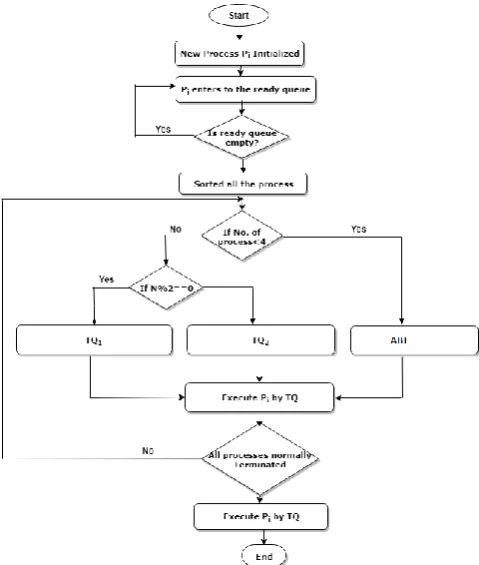
Fig. 1: Sequential working flow of the proposed algorithm
3.2 Proposed RR Algorithm
Figure 1 depicts the steps of the execution of the proposed algorithm. This flow chart shows how the algorithm works in sequentially. In this flowchart TQ1, TQ2 and ABT represent the equations (1), (2) and (3) where first two equations are used to calculate the time quantum and equation (3) is used to calculate the average burst time.
(1) (2) (3) The proposed algorithm is presented in the Algorithm 1. It showed how the time quantum is determined. If the numbers of processes are less than 4 then the time quantum is calculated from their average burst time which is shown in the line 5 to 9.
Algorithm 1: Proposed Round Robin Algorithm
1. Initialize: Ready Queue=0, Average Turn-around Time=0, Average Waiting Time=0, Time Quantum (TQ);
2. While(Ready queue != empty )
3. Sort all the Process in ascending order
4. N = number of process in the ready queue
5. If N <= 4
6. Sum ← 0 7. for i ← 1 to N do 8. Sum ← Sum + Pi
9. TQ ← Sum / N;
10. Else if (N%2 = 0)
11. TQ ← (Pi + PN + P(N/2) + P(N/2 + 1) )/4
12. Else
13. TQ ← (Pi + PN + P ceil( N/2 - 1) + P ceil(N/2 + 1) )/4
14. Executed the process by TQ
15. Calculate the average waiting time and average turn-around time
When the number of processes are more than 3 then the time quantum are determined for the odd and even number of processes which is shown in the line number 10 to 13. TQ will determine repeatedly until the burst time of all processes in the ready queue are zero as the proposed algorithm is dynamic. Finally the average turnaround time and average waiting time are calculated and the method is described in the below subsection which is working procedure.
3.3
Working
Procedure
The proposed algorithm is designed to meet all scheduling criteria such as maximum CPU utilization, maximum throughput, minimum turnaround time, minimum waiting time and minimum context switches. Three performance metrics: Turnaround Time (TAT), Waiting Time (WT) and Context Switching (CS) are considered in each case of our experiment.
(4) (5)
The proposed algorithm works on reducing the waiting time of the CPU process and enhancing CPU utilization. This algorithm combines with the features of SJF and Round Robin scheduling algorithm with varying time quantum which is described in the Algorithm 1. The algorithm is described step by step in below:
Initially, according to the proposed approach, the processes in the ready queue are arranged in the ascending order of their burst time.
For the different situations of ready queue, the algorithm runs different procedures to calculate the optimal time quantum.
When the number of processes present in the ready queue is less than or equal 4 then the time quantum has been taken by calculating the average of CPU processes burst time.
When the number of process (N) is even, then time quantum(TQ) is calculated by using equation (1).
Where Pi, PN, PN/2, and P(N/2+1) is the first process, last process, the median and thereafter present beside the median CPU process in the sorted ready queue.
When the number of process (N) is odd, then time quantum (TQ) is calculated by using equation (2).
Where, Pi, PN, P(N/2+1) and P(N/2-1) is the first, last, thereafter present beside the median and previous nearest of the median in the sorted ready queue.
For the different situations of CPU ready queue, the different time quantum is calculated dynamically.
repeated with the arrival of each process in the ready queue.
The time quantum is recalculated taking the remaining burst time after each cycle. In the next step, we have to rearrange the sorted processes along with all processes currently stored in a queue and repeat these systems again and again until the burst time of processes are zero.
3.4 Illustration
This subsection illustrated the methodology through an example to analysis the proposed algorithm which is described in the above subsection (Working Procedure). To demonstrate this procedure, a ready queue with eight processes P1, P2, P3, P4, P5, P6, P7, and P8 with their corresponding burst time 9, 10, 5, 12, 20, 14, 12 and 2 ms have been considered where the arriving time are 0, 4, 5, 5, 6, 8, 10, 10 ms respectively. When the arrival time is 0 ms, there has only process P1 reached in the ready queue. So, the time quantum is allocated according to P1 burst time and the time quantum is 9.
At 4 ms there have two processes in the ready queue those are P1 and P2. During this moment, the remaining burst time of P1 is 5. The processes P1 and P2 are arranged in the ascending order of their burst time in the ready queue which gives the sequence P1 and P2. Here the time quantum is counted in the average of those processes which is 8 and the shortest process executes first with this time quantum. After 1 ms there are P3 and P4 also in the ready queue. At that time the remaining burst time of P1 is 4. The arrangement of all the processes in the ascending order of their burst time in the ready queue gives the sequence P1, P3, P2, and P4. Averaging those processes burst time, the time quantum is 8 and the P1 is executed with this time quantum. After 1 ms, P5 also arrives in the ready queue. Due to having 5 (odd) possesses in the ready queue, the processes are arranged in the ascending order of their burst time in the ready queue which gives the sequence P1, P3, P2, P4, and P5. According to the condition of the proposed algorithm, the time quantum is calculated by the average of P1, P3, P4, andP5. The figured time quantum is 10 and P1 (smallest process) is executed with this time quantum. After 2 ms, P6 is in the ready queue and at that time, calculated the time quantum by taking P1, P2, P4, and P5 (according to the proposed algorithm). Now, the time quantum is 11. After 1 ms, the remaining burst time of P1 is 0 ms. So, by taking P3, P2, P6, and P5 the time quantum is 13. After 1 ms P7 and P8 are in the ready queue and the remaining burst time of P3 is 4. At that moment, taking P8, P2 P4, and P5 and the time quantum is 29. After 2 ms, P8 has been finished. Now the time quantum is 13 and after 4 ms, the remaining burst time of P3 is 0. According to the above description P2, P4, P7, P6, and P5 are executed with dynamic time quantum 14, 15, 16, 17 and 20. After executing the above procedure, the remaining burst time for all processes is 0 and the ready queue is empty. Figure 2 represents the Gantt chart of these procedures. Moreover, the calculated average waiting time 20.875 ms and the average turn-around time is 31.375 ms. Using the same set of the process with the same arrival and CPU burst times, the average waiting time is 37.25 ms and the average turnaround time is 47.75 in RR.
3.5 Theoretical Evaluation
Several researchers proposed new technique for the round robin algorithm to determine time quantum efficiently. However median, partial average and average are the three well-known methods used in this research to determine an optimal time quantum. This section presents the theoretical
explanation of the proposed algorithm.
Assume that the number of processes (P) in the ready queue is N. Now the time quantum for Median (M), Partial Average (PA) and Average (A) are:
M = (PN/2 + PN/2+1)/2
PA = (P1 + PN)/2
A= (P1 +P2 + P3 + …………+PN)/N
In the proposed algorithm, for N number of the process, the asymptotic analysis is:
TQ = (P1+PN/2+PN/2+1+PN)/4
= (P1/4 + PN/2 /4 + PN/2+1/4 + PN/4)
=1/2*((P1+PN)/2) + 1/2*((PN/2+PN/2+1)/2)
=1/2*PA+ 1/2*M
This analysis showed that when the Partial average method and median method show the best output independently, our proposed algorithm also shows a good result for containing both of them in one equation. Similarly at the case where the median method shows the worst result and Partial average shows the best result the proposed algorithm shows average good result for having both terms in the proposed equation and vice versa. When the few amounts of processes are in the ready queue, the system acts like the average time quantum method. So it also has benefits of average for some cases.
4.
RESULT AND DISCUSSION
4.1
Assumptions and Implementation
The proposed algorithm has been developed and illustrated with a view to increasing the performance of scheduling in the field of maximum throughput, maximum CPU utilization, reducing turnaround time and minimizing waiting time. Basically two type of processes such as having equal arrival time and different arrival time. In this research both of the cases are considered. The proposed algorithm had been implemented with C++ programming language with Core-i3 Processor, 4GB RAM, 64bit windows operating system computer. For conducting the experiment n processes have been taken and all of these are independent. Before executing the data of any test case for all the processes their corresponding burst time (BT) and arrival time (AT) are known. These are the input parameters of this system. The output parameters are average turnaround time (ATAT), average waiting time (AWT) and context switch (CS). Following sections describe about the datasets and experimental result obtained from the implemented system.
4.2
Datasets
The experiment has been conducted with two different test cases where one is with same arrival time and another is with different arrival time. The datasets have been selected randomly. Table 1 and 2 presents these datasets. To evaluate the performance of the proposed algorithm a comparative result has been conducted with two different data sets where the obtained result of our algorithm is presented with some selected algorithms proposed in the existing literature. This experiment also has been performed with two different datasets which shows in table 3 and table 5.
4.3
Experimental Result
Case 1: (Without arrival Time)
[image:5.595.320.537.73.162.2]Table 1 presents the first dataset where five processes have taken with their respective burst time with arrival time 0.
Table 1: Dataset- 1
Process Id CPU Burst Time (ms)
P1 22
P2 18
P3 9
P4 10
P5 5
[image:5.595.53.281.122.240.2]The Gantt chart of the proposed algorithm for the first dataset is demonstrated in Figure 2.
Fig. 2: Gantt chart for dataset 1
Proposed algorithm provides the following result for the first dataset: the number of Context Switches 4, average waiting time 13 ms average turnaround time 29.8 ms. Using the same set of the process with the same arrival and CPU burst times, standard RR provides a number of context switches 13, the average waiting time is 34 ms and the average turnaround time is 46.8 in RR where time quantum is 5.
Case 2: (With Arrival Time)
[image:5.595.58.272.284.335.2]Assume eight processes P1, P2, P3, P4, P5,P6, P7, andP8 arriving at different times 0, 4, 5, 5, 6, 8, 10 and 10 respectively with increasing burst time 9, 10, 5, 12, 20, 14, 12 and 2. Table 2 presents the details of this dataset.
Table 2: Dataset - 2
Process Id Arrival time CPU Burst Time (ms)
P1 0 9
P2 4 10
P3 5 5
P4 5 12
P5 6 20
P6 8 14
P7 10 12
P8 10 2
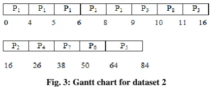
The Gantt chart of the proposed algorithm is demonstrated in Figure 3.
Fig. 3: Gantt chart for dataset 2
In this process, a number of context switches 12, average waiting time 20.875 ms, average turnaround time 31.375 ms. Using the same set of the process with the same arrival and CPU burst times, a number of context switches 14 in RR, the average waiting time is 45 ms in RR. The average turnaround time is 55.5 in RR (at time quantum 8).
From the above experiment context switch, average waiting time and average turnaround time both are reduced by using the proposed algorithm. The reduction of context switch, average waiting time and average turnaround time shows maximum CPU utilization and minimum response time. This proposed algorithm is much more efficient as compared to a simple RR algorithm.
4.4 Comparison with Algorithms
Two different data sets have been conducted to evaluate the proposed system by comparing some other existing methods. For ensure the effectiveness and accuracy of this proposed algorithm, some existing algorithms had been selected. The selected algorithms are listed below:
Dynamic Quantum Using the Mean Average Round Robin (ANRR) [5]
Shortest Remaining Burst RR (SRBRR) [6]
An Optimized Round Robin Algorithm (ORR)[7]
Adaptive Round Robin Algorithm (ARR) [8]
Simple Round Robin Algorithm (RR) [12]
Case 1:
[image:5.595.58.277.498.665.2]Assume six processes P1, P2, P3, P4, P5, and P6 arriving at different times 0, 0, 3, 5, 10, 13 respectively with burst time 7, 5, 4, 4, 8, 8 as shown in Table 3.
Table 3: Dataset 3
Process Id Arrival time Burst Time
P1 0 7
P2 0 5
P3 3 4
P4 5 4
P5 10 8
P6 13 8
[image:5.595.310.549.533.669.2]Table 4: Comparison over dataset 3
Algorithms ATAT AWT CS
RR (At TQ=4) 17.17 11.17 9 SRBRR 14.833 8.833 8
AN RR 15.83 9.83 6
ORR, TQ = 4 (Phase 1), 8 (Phase 2)
15.00 9.00 7
Adaptive RR 16.67 10.67 7
Proposed Algorithm 13.33 7.33 7
Case 2:
[image:6.595.49.288.78.229.2]Assume Five processes P1, P2, P3, P4, and P5 arriving at different times 0, 6, 8, 9, 10 respectively with burst time 7, 15, 90, 42 and 8 are shown in Table 5.
Table 5: Dataset 4
Process Id Arrival Time Burst Time
P1 0 7
P2 6 15
P3 8 90
P4 9 42
P5 10 8
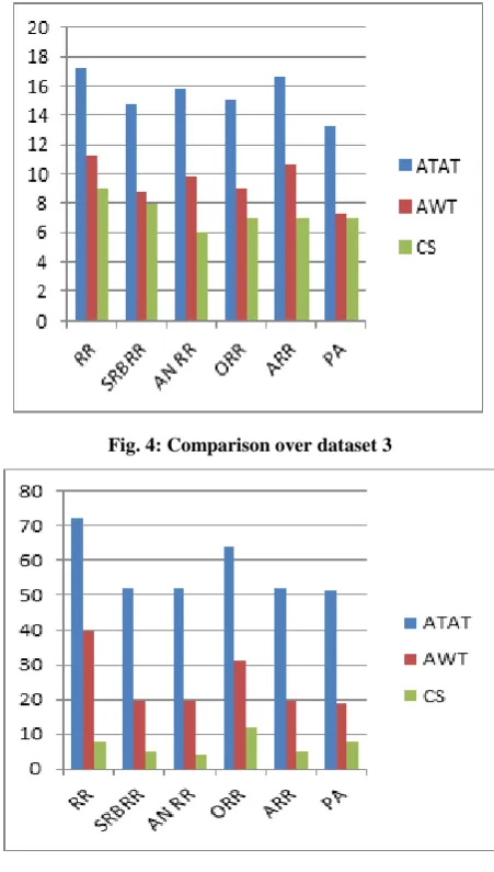
The result of the proposed algorithm against the mentioned algorithms has been shown in Table 6. The result shows that the proposed algorithm performs better than other algorithms in terms of ATAT, AWT. In the terms of CS some other algorithms show better performance than the proposed algorithm. Table 6 presents the details of the result and Figure 5 represents the comparison in a clear concise.
Table 6: Comparison over dataset 4
Algorithms ATAT AWT CS
RR (At TQ=25) 72 39.6 8
SRBRR 52 19.6 5
AN RR 52 19.6 4
ORR,TQ = 6 (Phase One), 12 (Phase Two), 24, 48
63.8 31.4 12
ARR 52 19.6 5
Proposed Algorithm 51.2 18.8 8
Fig. 4: Comparison over dataset 3
Fig. 5: Comparison over dataset 4
5.
CONCLUSION
[image:6.595.51.285.294.393.2]6.
REFERENCES
[1] Silberschatz, Abraham, Greg Gagne, and Peter B. Galvin. Operating system concepts. Wiley, 2018. [2] S. R. Chavan, P. C. Tikekar, An Improved Optimum
Multilevel Dynamic Round Robin Scheduling Algorithm, International Journal of Scientific & Engineering Research, Volume 4, Issue 12, December-2013 ISSN 2229-5518.
[3] Sukumar Babu B., Neelima Priyanka N., and Sunil Kumar B., "Efficient Round Robin CPU Scheduling Algorithm," International Journal of Engineering Research and Development, vol. 4, Ino. 9, Nov. 2012, p. 36-42.
[4] Ajit Singh, Priyanka Goyal, Sahil Batra, An Optimized Round Robin Scheduling Algorithm for CPU Scheduling, (IJCSE) International Journal on Computer Science and Engineering Vol. 02, No. 07, 2010, 2383-2385.
[5] Abbas Noon, Ali Kalakech and Seifedine Kadry, “A New Round Robin Based Scheduling Algorithm for Operating Systems: Dynamic Quantum Using the Mean Average,” International Journal of Computer Science, vol. 8, no. 1, May 2011, p. 224-229.
[6] Prof. Rakesh Mohanty, Prof. H. S. Behera, Khusbu Patwari, Manas Ranjan Das, Monisha Dash, Sudhashree, Design and Performance Evaluation of a New Proposed Shortest Remaining Burst Round Robin (SRBRR) Scheduling Algorithm.
[7] Ajit Singh, Priyanka Goyal, and Sahil Batra, "Optimized Round Robin Scheduling Algorithm for CPU Scheduling," International Journal on Computer Science and Engineering, vol. 02, no. 07, 2010, p. 2383-2385.
[8] Saroj Hiranwal and Dr. K.C. Roy, “Adaptive Round Robin Scheduling using Shortest Burst Approach Based on Smart Time Slice,” International Journal of Computer Science and Communication, vol. 2, no. 2, July-Dec. 2011, p. 319-323.
[9] Sukumar Babu B., Neelima Priyanka N., and Dr. P. Suresh Varma, "Optimized Round Robin CPU Scheduling Algorithm," Global Journal of Computer Science and Technology, vol. 12, Issue 11, 2012, p. 21-25.
[10]Sukumar Babu B., Neelima Priyanka N., and Sunil Kumar B., "Efficient Round Robin CPU Scheduling Algorithm," International Journal of Engineering Research and Development, vol. 4, Ino. 9, Nov. 2012, p. 36-42.
[11]Matarneh, Rami J. "Self-adjustment time quantum in round robin algorithm depending on burst time of the now running processes." American Journal of Applied
Sciences 6.10 (2009): 1831.
[12] Christopher McGuire and Jeonghwa Lee, Comparisons of Improved Round Robin Algorithms, Proceedings of the World Congress on Engineering and Computer Science 2014 Vol I WCECS 2014, 22-24 October 2014, San Francisco, USA.
[13] Bhavin Fataniya1, Manoj Patel2, Survey on Different Method to Improve Performance of The Round Robin Scheduling Algorithm, International Journal of Scientific Research in Science, Engineering and Technology.
[14] Mohanty, Rakesh, et al. "Priority based dynamic round robin (PBDRR) algorithm with intelligent time slice for soft real time systems." arXiv preprint arXiv:1105.1736 (2011).
[15] Salman Arif, Saad Rehman and Farhan Riaz "Design of A Modulus Based Round Robin Scheduling Algorithm", IEEE, 9th Malaysian Software Engineering Conference, Dec. 2015.
[16] Pandaba Pradhan, Prafulla Ku. Behera and B N B Ray, "Modified Round Robin Algorithm for Resource Allocation in Cloud Computing ", ScienceDirect, Procedia Computer Science (2016 ) 878 – 890,2016.
[17] Amar Ranjan Dash, Sandipta Kumar Sahu, and Sanjay Kumar Samantha, An Optimized Round Robin CPU Scheduling Algorithm with Dynamic Time Quantum, International Journal of Computer Science, Engineering and Information Technology (IJCSEIT), Vol. 5, No.1, February 2015.
[18] H.S.Behera, Rakesh Mohanty, Sabyasachi Sahu, and Sourav Kumar Bhoi, "Comparative Performance Analysis of Multi-dynamic Time Quantum Round Robin (mdtqrr) Algorithm with Arrival Time," Indian Journal of Computer Science and Engineering, vol. 2, no. 2, Apr-May 2011.
[19] Mohanty, Rakesh, et al. "Design and performance evaluation of a new proposed shortest remaining burst round robin (SRBRR) scheduling algorithm." Proceedings of International Symposium on Computer Engineering & Technology (ISCET). Vol. 17. 2010.
[20] Ghanbari, Shamsollah, and Mohamed Othman. "A priority based job scheduling algorithm in cloud computing." Procedia Engineering 50.0 (2012): 778-785.