Effectiveness of log-logistic distribution to model water-consumption data
1
2
Seevali Surendran1,2*and Kiran Tota-Maharaj1 3
4
1Faculty of Environment and Technology, University of the West of England, Bristol (UWE
5
Bristol), Bristol, BS16 1QY, UK; 2Environment Agency, Kings Meadow House, Kings 6
Meadow Road, Reading, RG1 8DQ, UK. *Corresponding author Email: 7
9
ABSTRACT
10
Water consumption varies with time of use, season and socio-economic status of consumers, and 11
is defined as a continuous random variable. Incorporating probabilistic nature in water-12
consumption modelling will lead to more realistic assessments of performance of water 13
distribution systems. Furthermore, fitting water-consumption patterns into a suitable statistical 14
distribution will assist in determining how often peaks will occur, or the probability of exceeding 15
the peaking factor in a system, for incorporation into design calculations. There are few studies 16
in the literature where the random variations of consumption have been considered. The purpose 17
of this study is to evaluate real water-consumption data from the United Kingdom (UK) and 18
North America and to investigate the possibility of establishing a standard probability 19
distribution function to apply in simulating water consumption in developed countries. Daily 20
water-consumption data for five years (2009–2013) were obtained from water companies in the 21
UK and North America and analysed by fitting into normal, log-normal, log-logistic and Weibull 22
distributions. Statistical modelling was performed using MINITAB version 18 statistical 23
package. The Anderson-Darling goodness-of-fit test was used to show how well the selected 24
statistical distribution fits the water-consumption data. 25
26
KEYWORDS | Anderson-Darling statistical test, log logistic distribution, MINITAB, 27
probability distribution function, random nature, water demand 28
INTRODUCTION
30
A major unresolved problem in water-consumption modelling is the identification of an 31
appropriate statistical distribution which best represents the water-consumption pattern. Fitting 32
water-consumption patterns into a suitable statistical distribution will assist in finding how often 33
the peaks will occur, or the probability of exceeding the peaking factor, in the system to 34
incorporate into design calculations with a scientifically proven method. The aim of this research 35
is to study real water-consumption data and to find a standard statistical distribution to use in 36
water-consumption modelling to address the probabilistic nature of water consumption. The 37
advantage of modelling real water-consumption data is that it will permit forecasting of the 38
probability of occurrence in any consumption value and provide confidence in future projections. 39
There are relatively few studies that have considered the random variations of water 40
consumption. It is often assumed that variation in water consumption in distribution systems 41
follows the normal distribution, usually with insufficient justification. Furthermore, there is 42
inadequate reliable data regarding the suitability of various statistical distributions for modelling 43
water consumption. Goulter and Bouchart (1990), Bao and Mays (1990), Xu and Goulter (1997, 44
1998, 1999), Syntetos et al. (2001, 2005) and Kwietniewski (2003) made assumptions that water 45
consumption has a normal distribution. Mays (1994) used randomly generated water-46
consumption data using a range of distributions to study the sensitivity of a system’s 47
performance to changes in water-consumption patterns. Khomsi et al. (1996) stated that the 48
consumption of water has a normal distribution based on the Kolmogorov-Smirnov test (KS). 49
However, the KS test is more sensitive near the centre of the distribution than at the tails and was 50
not suitable to validate the water-consumption data, as the high consumption data points lie on 51
the tail of the distribution. In the technical literature further research papers written by De 52
Marinis et al. (2007); Tricarico et al. (2007) and Gato-Trinidad and Gan (2012) support the 53
effectiveness of the normal distribution by means of rigorous statistical inferences on real data. 54
The American Water Works Association (AWWA) Research Foundation sponsored a study 55
(Bowen et al., 1993) in residential water-use patterns in the USA, and results revealed that the 56
demand data was not distributed normally. Several data transformations to improve the data 57
analysis were investigated and it was found that the log transformation was only mildly effective 58
Surendran and Tanyimboh (2004), and Tanyimboh et al. (2004) addressed the issue of the 60
modelling of short-term consumption variations in a comprehensive way, using UK water-61
consumption data and concluded that data fitted better with a long tail distribution rather than a 62
normal distribution. However, the findings were limited to UK water-consumption data. 63
The log-logistic distribution resembles the log-normal in shape, it has a more tractable 64
form and is one of the few distributions for which the probability distribution, cumulative density 65
and quartile functions exist in simple closed form (Kleiber, 2004). Furthermore, it can cope well 66
with outliers in the upper tail (Dey & Kundu 2004). The log logistic distribution has been used 67
by Swamee (2002), El-Saidi et al. (1990) and Rowinski et al. (2001), in hydrological studies 68
(frequency analysis of multi-year drought durations, precipitation data and flood frequency 69
analysis) and survival (reliability) analysis, which have the outliers in upper tail. Gargano et al. 70
(2016, 2017) stated that log-logistic distribution is the best fit for real water-consumption data. 71
Ashkar and Mahdi (2006), Cordeiro et al. (2012) and Ramos et al. (2013) described the 73
log-logistic distribution in detail and concluded that the log-logistic model is suitable for positive 74
skewed data and positive random variables. As water consumption is a random variable and is 75
positively skewed, it defines the suitability of log-logistic distribution in modelling water 76
consumption. 77
78
Identifying a suitable statistical distribution
79
It is a general assumption that water consumption follows a normal distribution and literature 80
review shows that the studies undertaken in the past supported this assumption. Water 81
consumption will vary as a result of weather patterns, fire incidents and leakages, and these 82
scenarios will lead to extreme usage conditions. Consequently, due to high consumption from 83
time to time, the data would fit better in a positively skewed distribution than in a normal 84
distribution 85
As a preliminary check, to identify the distribution patterns of the real water-consumption 86
data obtained from the two water companies, normal graphs were drawn to check the normality 87
of the data. The normal graphs were drawn for the 20 data sets (yearly data) and they show that 88
out of 20 data sets, 2 sets follow a normal distribution and the other 18 sets follow a positively 89
skewed distribution. 90
It can be concluded that water-consumption data will fit well into positively skewed distributions 91
such as log-normal, log-logistic and Weibull distributions. 92
This study used these distributions to select the best fit for water-consumption modelling. 93
The normal distribution was used for comparison. These four distributions are described in Table 94
1, providing their suitability on application to modelling water consumption. 95
96 97
Table 1. Suitability for using normal, log-normal, log-logistic and Weilbull distributions in 98
modelling 99
Distribution Description Suitability for water-consumption data modelling
Probability distribution function (PDF)
Normal Has the familiar symmetrical bell shape and its sample space extends from minus to plus infinity.
The water-consumption data contains only positive values and since the data typically show skewed frequency patterns, the
− − −
= x x
x f 2 2 1 exp 2 1 ) (
normal distribution must be approached with caution, particularly if inferences will focus on the tails of the distribution.
the standard deviation.
Log-normal Logarithmically related to normal distribution and shows considerable flexibility of shape, which is always skewed to the right.
In log-normal distribution its sample space admits only positive values and suitable to use in analysing water-consumption data.
(ln ) , , 0
2 1 exp 2 1 ) ( 2
2
− − =
x x x
x
f where is the mean and is the standard
deviation.
Log-logistic The log-logistic distribution resembles the log-normal in shape, has a more tractable form. It can cope well with outliers in the upper tail.
It is a uni-model, defined only for positive random variables and positively skewed which is best representing the water consumption pattern.
f(t)= lk(lt)
k-1
[1+(lt)k]2 t0
where is called a shape parameter, as
increases the density become more peaked. The parameter is a scale parameter.
Weibull Depending on the values of the parameters, the Weibull distribution can be used to model a variety of life behaviors and provides better distribution for life length data.
To use Weibull distribution in analysis, it is essential to have a very good justifiable estimate for the shape parameter to replicate the accurate distribution pattern.
where β is the shape parameter and η is the scale parameter.
100
Description of data and the relative water distribution systems
101
The daily water-consumption data for the five years from 1st April 2009 to 1st April 2013 were 102
obtained from a water utility company in North West Region of England to use in this research. 103
The water works system delivers water to approximately 6.7 million households and businesses 104
in the UK. The data were collected at the supply end of the network system using flow meters 105
which are either connected to telemetry (which are live) or data loggers. The data loggers record 106
the flow rate during the 15-minute period, depending on the pulse setting (i.e. how many litres 108
per pulse). This raw data is imported daily into the data management system and converged to 109
hourly and daily volumes. 110
To analyse the North American daily water consumption, data for three demand zones 111
from a Canadian city in Manitoba Province were obtained. The data were collected using flow 112
meters connected to data loggers at the water treatment plant by the water services division. The 113
data were received between 1st January 2009 and 31st December 2014. The water supply system 114
delivers an average of 225 million liters per day of water to approximately 270,000 households 115
and businesses across approximately 297 square kilometers (114 square miles) of developed area 116
in Canada. 117
118
METHODOLOGY
119
In this research, a suitable statistical distribution was selected using a descriptive analysis. Data 120
were screened and sorted by plotting raw demand data against time. This provided a quick 121
reference to check the abnormality of data. If the points were homogeneously distributed and 122
there were no negative points, this meant that the data were all most acceptable to use in the 123
analysis. Similarly, if there were any inconsistencies in the distribution, these time series graphs 124
would show the abnormal data points to be removed prior to analysis. 125
The data were then analysed using MINITAB version 18 statistical package, and was 126
fitted into a suitable probability distribution. As previously described, the descriptive analysis 127
show that data fit well into a positively skewed distribution and normal, Weibull and log-128
logistic distributions were applied to find an appropriate distribution. The normal distribution 129
was used for comparison purposes. 130
131
Analysing data
132
Once data has been fitted in to any distribution, the ‘goodness-of-fit test’ should be used to see 133
how well the data fit into the distribution. The parameters of distribution such as location, shape 134
and scale are also essential to describe the distribution. 135
136
The appropriateness of the distribution for water-consumption data was assessed by comparison 138
to the normal, log-normal, log-logistic and Weibull distributions using the Anderson-Darling 139
goodness of fit test. The Anderson-Darling Test (Stephens, 1974) is used to test if a sample of 140
data came from a population with a specific distribution. It is a modification of the K-S test and 141
gives more weight to the tails than the K-S test. The K-S test is distribution free in the sense that 142
the critical values do not depend on the specific distribution being tested. The Anderson-Darling 143
Test makes use of the specific distribution in calculating critical values. This has an advantage of 144
allowing a more sensitive test and the disadvantage is that critical values must be calculated for 145
each distribution. The critical values were calculated, tabulated and published by Stephens 146
(1974), for a few specific distributions, including log-logistic distribution. 147
The equation for the Anderson-Darling parameter, A2, is 148 149
(
)
= − + − + − − − = n i i n i i n n A 1 12 1 2 1 ln ln(1 )
150
where, n is the number of observations and i is the value of the distribution in question at the ith
151
largest observation. A smaller AD value indicates that the distribution fits the data better. The 152
critical value of the Anderson-Darling parameter at the 95% confidence interval is 2.492 the 1% 153
point is 3.857 for n≥5 (Johnson, 2000). The Anderson-Darling test was preferred to the 154
Kolmogorov-Smirnov test because of the latter’s lack of sensitivity in tails (Ahmad et al., 1988; 155 Johnson, 2000). 156 157 Parameter estimates 158
The location and scale parameters are associated with central tendency and dispersion, 159
respectively, and are essential to describe the distribution. The parameters for normal distribution 160
are the mean and standard deviation and they are directly related to the location and scale 161
parameters (Rigby, 2004). The log-normal, log-logistic and Weibull distributions use location, 162
shape or scale as their parameters and unlike normal distribution they need to transform the 163
location and scale parameters to represent mean and standard deviation using complex equations. 164
These parameters have allowed the distribution to have flexibility and effectiveness in modelling 165
applications. In simple terms the shape parameter allows a distribution to take on a variety of 166
shift the graph to the left or right of the horizontal axis. The scale parameter describes the 168
stretching capacity of the probability distribution function. 169
170
The graphical method 171
There are various numerical and graphical methods used in the literature for estimating the 172
parameters of a probability distribution. In this study, graphical methods were selected for the 173
analysis along with the maximum likelihood method to draw the probability plots (see Figures 1 174
and 2 in the following section). The data were analysed using 95% confidence intervals (5% 175
significance level) and were fitted to normal, log-normal, Weibull and log-logistic distributions 176
to establish the parameters for the distribution. The middle line in the probability plot shows the 177
normal line and the other two lines show the 95% confidence intervals. Montgomery and Runger 178
(2002) stated that normal probability plots are useful in identifying distributions that fit into the 179
normal distribution and those which have skewed distributions with long tails. If the data falls 180
below the normal line then data has a positively skewed distribution (Montgomery & Runger, 181
2002). 182
183 184
RESULTS AND DISCUSSION
185
The normal probability plots for the UK and North American water-consumption data for the 186
year 2009 is shown in Figure 1and Figure 2, respectively. The data shown in Figure 1 and Figure 187
2 shows that values on both ends tend to fall below the normal line. This demonstrates that the 188
data has a positively skewed distribution. Further to this, the graphs of four distributions for the 189
UK and North American data show that more data points are within the 95% confidence level for 190
192
[image:9.612.57.524.73.541.2]193 194
Figure 1. Probability plots for normal, log-normal, log-logistic and Weibull – UK 195
197
Figure 2. Probability plots for normal, log-normal, log-logistic and Weibull – North American 198
data. 199
200 201
The goodness-of-fittest
202
The Anderson-Darling (AD) goodness-of-fit test was used to confirm the best fit of data for 203
normal, normal, logistic and Weibull distribution. The AD values for normal, log-204
normal, log-logistic and Weibull distributions for the UK and North American data are shown in 205
Figures 3 to 6. The data used in this study has shown that the log-logistic distribution has the 206
208
Figure 3. Anderson-Darling (AD) test values – UK. 209
210
211
[image:11.612.70.491.364.568.2]213
Figure 5. Anderson-Darling (AD) test values for Zone 2 – North America. 214
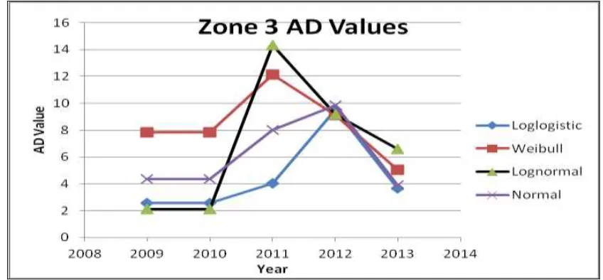
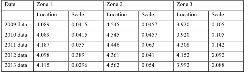
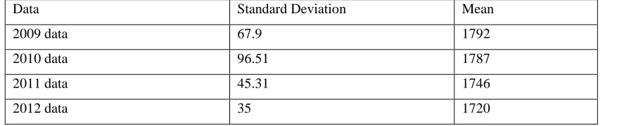
215 216
217
Figure 6. Anderson-Darling (AD) test values for Zone 3 – North America. 218
219 220
Parameter estimates
221
The location and scale parameters are associated with central tendency and dispersion, 222
respectively, and are essential to describe the distribution. The parameters for normal 223
distribution are the mean and standard deviation and they are directly related to the location and 224
scale parameters (Rigby, 2004). The log-normal, log-logistic and Weibull distributions use 225
[image:12.612.67.491.329.526.2]the location and scale parameters to represent mean and standard deviation using complex 227
equations. 228
These parameters have allowed the distribution to have flexibility and effectiveness in 229
modelling applications. In simple terms the shape parameter allows a distribution to take on a 230
variety of shapes depending on the value of the shape parameter. The effect of the location 231
parameter is to shift the graph to the left or right on the horizontal axis. The scale parameter 232
describes the stretching capacity of the probability distribution function. 233
The location parameter obtained in this study for the log-logistic distribution is 234
approximately 7.4 for the UK’s water-consumption data. The scale parameter is in between 235
0.0107 and 0.026 (Table 2). With regard to the North American water-consumption data, the 236
location parameter obtained for log-logistic distribution is between 3.92 and 4.562. Similarly, the 237
scale parameter is between 0.0296 and 0.389 (Table 3). The standard deviation is in a range of 238
1720 to 1792 and mean value is 35 to 96.51 for the UK’s consumption data (Table 4). 239
[image:13.612.78.540.380.483.2]240
Table 2. Location and scale parameters for log-logistic distribution for UK water demand data 241
Date Location Scale
2009 data 7.485 0.01776
2010 data 7.482 0.0256
2011 data 7.464 0.01517
2012 data 7.448 0.01068
242
Table 3. Location and scale parameters for log-logistic distribution for Canadian water demand 243
data 244
Date Zone 1 Zone 2 Zone 3
Location Scale Location Scale Location Scale
2009 data 4.089 0.0415 4.545 0.0457 3.920 0.105
2010 data 4.089 0.0415 4.545 0.0457 3.920 0.105
2011 data 4.187 0.055 4.446 0.063 4.308 0.142
2012 data 4.098 0.389 4.361 0.041 4.152 0.092
2013 data 4.115 0.0296 4.562 0.054 3.992 0.088
[image:13.612.64.499.542.668.2]248
Table 4. Standard deviation and mean values for water-consumption data for UK water demand 249
Data Standard Deviation Mean
2009 data 67.9 1792
2010 data 96.51 1787
2011 data 45.31 1746
2012 data 35 1720
250
CONCLUSIONS
251
It was observed that by analysing water-consumption data, 88% of the water-consumption data 252
has a positively skewed distribution. This means that data would fit better for positively skewed 253
distributions such as log-normal, log-logistic and Weibull. Following detailed analysis of data, 254
the study shows that from the four selected distribution patterns studied, the log-logistic 255
distribution provided the lowest AD values and was the most suitable water-distribution pattern 256
to standardise when modelling the water demand. 257
The findings in this study are in accordance with the literature which stated that log-258
logistic distribution is the best fit for real water-consumption data. Although log-normal and 259
log-logistic distributions may be similar for moderate sample sizes, it is still desirable to choose a 260
more suitable model to obtain an accurate probability values at tails. 261
Moreover, the normal and log-normal distributions produced marginally acceptable AD 262
values. The AD values obtained for the Weibull distribution have higher values when compared 263
with the other three distributions (log-logistic, log-normal and normal) and were found not to be 264
suitable in simulating the water demand data. 265
To the best of the authors’ knowledge, there are no prior studies which have incorporated 266
the probability of occurrence using real water-consumption data built upon a statistically 267
analysed method focused on the upper tails. Using AD test to validate the data, this study 268
focused on the data on upper tails which best represents the water-consumption data. 269
The log-logistic distribution could be used as a standard statistical distribution in 270
quantifying the probability of exceedence of the water consumption. Additionally, this work also 271
has the potential to provide, significant information to help policy makers forecast future 272
demands using a fully probabilistic method. 273
ACKNOWLEDGEMENTS
275
The authors wish to express their gratitude to the Environment Agency for supporting this 276
research initiative, and water utility companies from the UK and North America for providing 277
the data sets for this study. 278
279
REFERENCES
280 281
[1] Ahmad, M. I., Sinclair, C. D. & Spurr, B. D. (1988) Assessment of flood frequency 282
models using empirical distribution function statistics. Wat. Resour. Res. 24 (8), 1323-283
1328 284
285
[2] Ashkar F and Mahdi S, (2006). Fitting the log-logistic distribution by generalized moments. 286
Journal of Hydrology, 328, 694-703 287
[3] Bao, Y. and Mays, L.W., (1990). Model for water distribution system reliability. J. of 288
Hydraul. Eng., Vol.116(9), 1119-1137 289
[4] Bowen P T, Harp J F, Baxter W J and Shull R D, (1993). Residential water use patterns. 290
American Water Works Association - Research Foundation, USA. 291
[5] Cordeiro G M, Santana T V F, Ortega E M M and Silva G O. (2012). The 292
Kumaraswamy-LogLogistic distribution. Journal of Statistical Theory and Applications, 293
11, 265-291. 294
[6] De Marinis, G., Gargano, R. and Tricarico, C. (2007). Water demand models for a small 295
number of users. ASCE Proceedings of the 8th Annual International Symposium on 296
Water Distribution Systems Analysis, Cincinnati, OH, doi: 10.1061/40941(247)41. 297
[7] Dey, A. K. & Kundu, D. (2004), Discriminating between Log normal and Log logistic 298
distributions, Journal of Statistical Computation and Simulation vol.74, no.2, 107–121. 299
[8] El-Saidi M A, Singh K P and Bartolucci A A. (1990), A note on a characterisation of the 300
generalised log-logistic distribution. Environmetrics; 1 (4), 337-342. 301
[9] Gargano, R.; Tricarico, C.; Del Giudice, G.; Granata, F. (2016). A Stochastic Model for 302
Daily Residential Water Demand. Water Sci. Technol. Water Supply 2016, 16, 1753-303
1767. 304
[10] Gargano, R., Tricarico, C., Granata, F., Santopietro, S., de Marinis, G. (2017). 305
Probabilistic Models for the Peak Residential Water Demand. Water (Switzerland), 9, 306
417. 307
[11] Gato-Trinidad, S. and Gan, K., (2012). Characterizing maximum residential water demand. 308
Urban Water - WIT Transactions on The Built Environment, Vol.122, 15-24. 309
310
[12] Goulter I C and Boulchart F, (1990). Reliability constrained pipe network model, Journal 311
of hydraulic engineering, ASCE, 116, (2), 211- 227. 312
[13] Johnson R A, (2000). Probability and statistics for Engineers, Prentice Hall, London. 313
[14] Khomsi D, Walters G A, Thorly A R D and Ouazar D, (1996). Reliability tester for water 314
distribution networks, Journal of Computing in Civil Engineering, ASCE, 10, (1), 11-19. 315
[15] Kleiber C (2004). ‘Lorenz ordering of order statistics from log-logistic and related 316
[16] Kwietniewski M, (2003). ‘Reliability Modelling of Water Distribution System (WDS) for 318
Operation and Maintenance Needs’, Journal of Hydro-Engineering and Environmental 319
Mechanics Vol. 51 (2004), No. 1, pp. 85–92. 320
[17] Mays L W, (1994). Computer Modelling of Free Surface and Pressurised flows, 321
Chaudray M H and Mays L W (editors), Kluwer Academic Publishers, Netherland, 485-322
517. 323
[18] Montogomary D C and Runger G C, (2002). ‘Applied statistics and probability for 324
Engineers’, 3rd edition, Printed in USA.
325
[19] Ramos M W A, Cordeiro G, Marinho P, Dias C (2013).The Zografos-Balakrishnan Log-326
Logistic Distribution: Properties and Applications, Journal of Statistical Theory and 327
Applications, Vol. 12, No. 3 (September 2013), 225-244 328
[20] Rowinski P M, Strupczewski W G and Singh V P (2001), ‘A note on the applicability of 329
log-Gumbel and log-logistic probability distributions in hydrological analyses’: I. 330
Hydrological Sciences Journal, 47 (1), 107-122. 331
[21] Stephens M A (1974), ‘EDF statistics for goodness of fit and some comparisons’, J. 332
American Statistical Association, Vol.69, pp. 730-737. 333
[22] Surendran, S., Tanyimboh, T. and Tabesh, M. (2005). Peaking demand factor-based 334
reliability analysis of water distribution systems. Advances in Engineering Software, 335
36(11-12), pp.789-796.96. 336
[23] Swamee, P.K. (2002). Near lognormal distribution. J. Hydrol. Eng., 7(6), 441-444. 337
[24] Syntetos A. A. & Boylan, J E, (2001). On the bias of intermittent demand estimates. 338
International Journal of Production Economics, 71, 457– 466. 339
[25] Syntetos A.A, and Boylan, J E, (2005). The accuracy of intermittent demand estimates, 340
International Journal of Forecasting 21 (2005) 303– 314 341
[26] Tanyimboh T T and Surendran S, (2002). Log-logistic Distribution Models for Water 342
Demands, 4th International Conference on Engineering and Technology Civil-Comp 343
press, Sterling. 344
[27] Tricarico, C., de Marinis, G., Gargano, R. and Leopardi, A., (2007). Peak residential water 345
demand. Water Management Journal, Vol.160(WM2), pp.115-121. 346
347
[28] Xu C and Goulter I C, (1997). A New model for reliability based optimal design of water 348
distribution networks, The 27th Congress of the International Association for Hydraulic 349
Research, ASCE, 423-428. 350
[29] Xu C and Goulter I C, (1998). Probabilistic model for distribution reliability, Journal of 351
Water Resources Planning and Management, ASCE, 124, (4), 218-228. 352
[30] Xu C and Goulter I C, (1999). Reliability based optimal design of water distribution 353
networks, Journal of Water Resources Planning and Management, ASCE, 125, (6), 352-354
362. 355