Human well being and in work benefits : a randomized controlled trial

Original citation:

Dorsett, Richard and Oswald, Andrew J. (2014) Human well-being and in-work benefits : a randomized controlled trial. Working Paper. Coventry, UK: Department of Economics, University of Warwick. (Warwick economics research papers series (TWERPS)).

Permanent WRAP url:

http://wrap.warwick.ac.uk/59377

Copyright and reuse:

The Warwick Research Archive Portal (WRAP) makes this work of researchers of the University of Warwick available open access under the following conditions. Copyright © and all moral rights to the version of the paper presented here belong to the individual author(s) and/or other copyright owners. To the extent reasonable and practicable the material made available in WRAP has been checked for eligibility before being made available.

Copies of full items can be used for personal research or study, educational, or not-for-profit purposes without prior permission or charge. Provided that the authors, title and full bibliographic details are credited, a hyperlink and/or URL is given for the original metadata page and the content is not changed in any way.

A note on versions:

The version presented here is a working paper or pre-print that may be later published elsewhere. If a published version is known of, the above WRAP url will contain details on finding it.

HUMAN WELL-BEING AND IN-WORK BENEFITS: A

RANDOMIZED CONTROLLED TRIAL

Richard Dorsett, Andrew J. Oswald

No 1038

WARWICK ECONOMIC RESEARCH PAPERS

HUMAN WELL-BEING AND IN-WORK BENEFITS: A RANDOMIZED CONTROLLED TRIAL

Richard Dorsett*, Andrew J. Oswald

February 2014

Abstract

Many politicians believe they can intervene in the economy to improve people’s lives. But can

they? In a social experiment carried out in the United Kingdom, extensive in-work support was

randomly assigned among 16,000 disadvantaged people. We follow a sub-sample of 3,500

single parents for 5 ensuing years. The results reveal a remarkable, and troubling, finding. Long

after eligibility had ceased, the treated individuals had substantially lower psychological

well-being, worried more about money, and were increasingly prone to debt. Thus helping people

apparently hurt them. We discuss a behavioral framework consistent with our findings and

reflect on implications for policy.

JEL codes: I31, D03, D60, H11, J38.

*Corresponding author: Richard Dorsett, National Institute of Economic and Social Research, 2 Dean Trench Street, Smith Square, London SW1P 3HE, UK; email: [email protected].

Word count (excl Tables and references): 6,047

Acknowledgements

HUMAN WELL-BEING AND IN-WORK BENEFITS: A RANDOMIZED CONTROLLED TRIAL

“Statistical offices [worldwide] should incorporate questions to capture people’s life evaluations, hedonic experiences and priorities.” p.16. Executive Summary of the Stiglitz-Sen-Fitoussi Commission Report on the Measurement of Social and Economic Progress, 2009. www.stiglitz-sen-fitoussi.fr

“There is ... a tendency to regard any existing government intervention as desirable.” Milton Friedman, Capitalism and Freedom, University of Chicago Press, 1962.

1. Introduction

Economic and social policies in western society are rarely based on the kinds of evidence

required in fields such as medical science. How high to set the income-tax rate, whether to pay

generous assistance to unemployed workers, what sorts of divorce laws to implement, how to

regulate banks -- these types of decisions have been shaped historically by politicians’ intuitions

and the lobbying of advisors. By building upon new strands within the quantitative

social-science literature, particularly research on well-being (Di Tella et al. 2001; Easterlin 2003;

Stiglitz et al. 2009; Oishi et al. 2012; Adler and Posner 2008; Ifcher 2011; Ifcher and Zarghamee

2011; Dolan and Metcalfe 2012; Layard 2006; Helliwell and Huang 2008; Benjamin et al. 2012;

Graham and Nikolova 2013; Stevenson and Wolfers 2013; Oswald et al. 2014), and upon

insights from an important modern literature on randomized trials (Burtless 1995; Gintis 2000;

Harrison and List 2005; List 2006; Dunn et al. 2008; Ludwig et al. 2011), this paper is an

attempt to pursue an alternative approach of evaluation by randomized controlled trial. The

analysis links also to issues of self-control (Thaler and Shefrin 1981). We study a major

social-science experiment run by the government of the United Kingdom -- a randomized controlled

trial that offered incentives to disadvantaged people to remain and advance in work and to

policies are discussed in Pencavel 1986, Eissa and Hoynes 2004, Bargain and Orsini 2006, and

Brewer et al. 2009).

Our main finding is that the intervention led to significant falls -- when measured after 5

years -- in the reported well-being levels of those people in the treatment group even though on

average those individuals ended with higher earnings than the control group. People became

less happy with their lives and worried more. Six well-being measures are available in our data

set. Because of the multiple-comparisons problem of applied statistics, and to obviate the need

for Bonferroni or equivalent corrections, results for all six measures are presented in the main

body of the paper or in the Appendix (which is divided into three sections, A, B, and C).

Each of the six measures points to substantially lower well-being. In four of these the

negative effects are individually significantly different from zero at the 1% or 5% significance

levels. The randomized intervention had no discernible effects on hours worked (measured at

Year 5). Hence no detailed tables are given later on that dimension of behavior. They are

available upon request. Because earnings increased in the treatment group, the treated

individuals could be said to be in higher-effort, or better, jobs. We return to this below.

As part of the study, we checked that the observable demographic characteristics of the

treatment and control groups had not altered in Year 5. A later part of the Appendix also tests

for the possibility of attrition bias caused by unobservables.

Why was the well-being of the treatment group reduced by the policy? That is a

fundamental puzzle for social scientists and remains to be completely understood. One

possibility, in the broad spirit of prospect theory (Kahneman and Tversky 1979), is that the

removal of temporary state benefits hurts asymmetrically more than the initial gain from those

criminality, in early research described in McCord (2007). One later section of our paper

explores the structure of a formal account. A section of the Appendix also summarizes different

reactions within the treatment group.

2. The Nature of the Randomized Trial

In the experiment (known as the Employment and Retention Advancement, or ERA,

Demonstration), individuals were assigned in a randomized controlled trial to one of two groups

-- either to a treatment group who were given additional incentives and support to take full-time

work or to a control group who were not. In total, approximately 16,000 individuals were

initially randomized, making this the largest social experiment undertaken in the UK (Hendra et

al. 2011; Haynes et al. 2012). The results in this paper focus on a random sub-sample of 3,500

single mothers followed up in telephone and face-to-face interviews both at 2 years and at 5

years after the initial policy intervention. There were a small number (3%) of single fathers in

the sample of single parents; for reasons of simplicity and homogeneity of sample these are

omitted from the later calculations. If the single fathers are included in the later analysis, it

makes no substantive difference to the study’s conclusions. No survey data for Year 5 were

collected on the remaining 12,500 people. That is why our study is of single mothers.

We draw in part upon a tradition of research -- across the fields of psychology, decision

science, medical science, economics, and other behavioral sciences -- that uses questionnaire

data on people’s well-being. These usually take the form of numerical scores in response to

survey questions such as: “how happy are you with your life overall” or “did you yesterday have

moments of anxiety or of feeling depressed”? Sample sizes in published statistical analyses vary

from a few dozen individuals in a laboratory to hundreds of thousands of people in a household

of a match between objective and subjective scores. This study focuses particularly upon

life-satisfaction data. Other forms of well-being and positive-affect information can be used (Stone

et al. 2010; Oswald and Wu 2010). Our later tables lay out results for a range of subjective

scores such as the level of worry about debt.

For clarity, some of this paper’s detailed tables are relegated to an Appendix. The key

statistical results of the study are presented in Tables 1 and 2.

Outcomes in Year 5 are of special interest, so they are our focus in this paper. There are

two reasons. One is that some payments were still being made to the experimental subjects at the

end of the second year, which thus complicates inference in Year 2. By the fifth year, however,

all payments and assistance to the treatment group had stopped. Hence Year 5 allows a clean

comparison. A second reason is that a major question for the western governments is: can a

policy of temporary in-work support help to foster long-run psychological and economic gains

for their citizens?

In this paper the treated subjects are compared to equivalent people in the control group

of that year. The conclusions are the following. First, the treatment increased Year-5 earnings

and, for an initial period before Year 5, the chance of being in full-time work. Table I

summarizes the economic outcomes. The ERA intervention raised people’s earnings, five years

afterwards, by approximately 10 pounds (about 15 US dollars) per week. In this sense, the

results are more positive than some found earlier (Foley and Schwartz 2003; Card and Hyslop

2009). They are also slightly more positive than the key earnings impacts in the official

evaluation report (Hendra et al. 2011) – see Section 1 of the Appendix for further details.

However, the principal contribution here is to attempt to go beyond pecuniary consequences to

treatment had no statistically significant effects on people’s hours worked. The point estimate,

when comparing the treatment group with the control group, was 0.8 extra hours a week, with a

large standard error (at Year 2, the effect was approximately one and half hours, significant at the

5% level). This finding continued to hold with tobit and other estimation methods. Hence, the

later sections do not attempt to report detailed results for hours worked. Second, when compared

to the control group, after five years the people who had been randomly assigned to the ERA

treatment group had substantially lower satisfaction with their lives, perceived their financial

situation as worse, ran out of money more often, worried about money to a greater extent, had

more trouble with debts, and were less likely to have money left over at the end of the week.

These were the individuals who were given extra public money and assistance. Helping them

apparently hurt them.

<Table I>

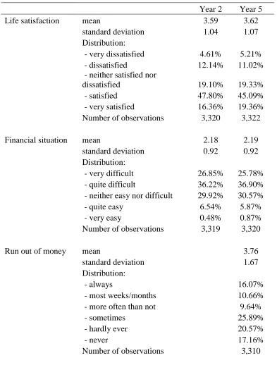
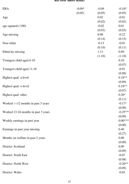
Table II gives the randomized trial’s key outcomes (other detailed findings are in the

Appendix). The negative effect on life satisfaction in Year 5 is approximately -0.1 points. That

drop relative to the control group is substantial. It is -- see Appendix A -- approximately half the

size of the effect of having no educational qualifications compared to having passed advanced

high-school exams. Life satisfaction in the econometric analysis is measured on a cardinal

five-point scale. However, switching to ordinal estimators such as probit equations makes no

substantive difference. The mean level of life satisfaction in Year 5 is 3.62 with a standard

deviation of 1.07. It might be felt that a 0.1 effect is reasonably small. But such intuition would

be misleading because the standard deviation here is driven by people’s cross-sectional variation

in answers. In fact, the in-work support made available under ERA apparently created

Table II suggests that the negative consequences work principally through greater

financial worries. One potential interpretation is that giving people temporary subsidies in Year

1 and Year 2 created aspirations and a lifestyle that were impossible to sustain.

<Table II>

3. The Intervention in Greater Detail

Individuals in the treatment group were given help in three broad ways. First,

participants in ERA had access to special ‘post-employment’ job coaching. Second, they were

given strong financial incentives to work. Third, they were given training opportunities. All

these were added, in effect, to the standard benefits available to anyone in the UK and to the job

placement services ordinarily available through unemployment offices. The intervention was

designed to add to the understanding achieved from experimental research carried out in the US

and Canada (Foley and Schwartz 2003; Card and Hyslop 2009; Rangarajan and Novak 1999;

Gennetian et al. 2005; Huston et al. 2003; Michalopoulos et al. 2002; Hendra et al. 2010).

The job coaching available under the ERA experiment took the form of advice and

assistance from an 'Advancement Support Adviser', specially trained to help individuals remain

and advance in work. Those who did so could receive substantial cash rewards, called ‘retention

bonuses’. These formed a key element of the ERA support (Dorsett and Robins 2014). They

were based on a 17-week accounting period. Individuals working 30 hours or more per week for

13 out of 17 weeks received a tax-free payment of £400. This works out at about £1 per hour for

an individual working 30 hours a week for just 13 weeks. It can be compared to an average

hourly wage of about £8 for those in work at the time of the year-5 survey interview (Hendra et

al. 2011). This is approximately 12.5%. Each individual could receive a maximum of six

point for everyone in the treatment group, regardless of what use they had made of the support

on offer. Lastly, ERA encouraged training by providing help with tuition costs and offering cash

rewards for completing training courses while employed.

A number of steps were taken to ensure a high response rate and to keep track of

respondents. Respondents were given a £20 voucher in return for their cooperation. Individuals

in the survey sample were sent pre-contact letters (first done 6 months after the randomization)

setting out the purpose of the study and the survey, explaining about the £20, giving a

confidentiality assurance, and enclosing a postcard to inform of changes in contact details.

Another letter was sent 8 days before the start of fieldwork. Interviewing was managed by the

Office of National Statistics and was carried out by telephone, with non-contacts and refusals

re-issued to face-to-face interviewers. Details were recorded of 3 other people who could be

approached in case there were difficulties contacting the person.

Prior to the randomization, information was collected on individuals’ baseline

characteristics. People’s subsequent employment, earnings and welfare outcomes were tracked

by using a mixture of administrative records and surveys. Three surveys were carried out --

approximately one, two and five years after randomization. The timing of these surveys was

such that the first two fell within the period of ERA eligibility, while the last survey, held in

year 5, was a substantial period after all ERA participation and payments had ended. This timing

allows the effects of ERA -- both during and beyond the period of eligibility -- to be examined.

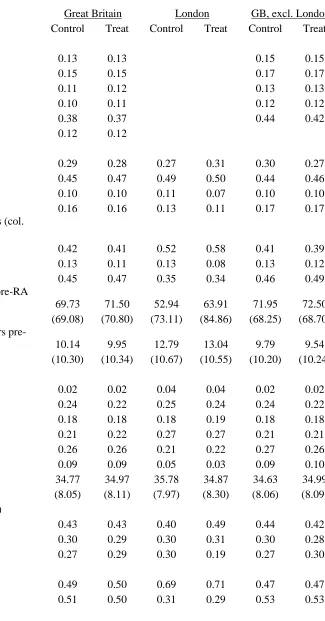
Appendix Table A.1 describes basic background information about the sample used in

the calculations. The characteristics of the participants in (both of) the Year 2 and Year 5

surveys are shown. In total, the sample consists of 3,335 respondents. At the start of the study

Approximately 40% of participants had worked for fewer than 12 months out of the previous 36

months. Importantly, it can be seen from Table A.1 that the mean characteristics of the

treatment group and the control group are almost identical. Some differences are to be expected

as a result of random variation, particularly as smaller subsamples are considered. For example,

the third and fourth columns of Table A.1, which give data for the area of London on its own,

show weekly earnings prior to randomization to differ between the control and treatment groups

(the means are 52.94 and 63.91 pounds). However, the difference falls short of statistical

significance at conventional levels (a two-tailed t-test gives a p-value of 0.175).

Some of the paper’s calculations are carried out for the regions of the UK excluding

London. The reason for wishing to do this is that market wages are typically considerably higher

in London than elsewhere, so the retention bonuses paid to the treatment group as part of the

ERA experiment represent a considerably greater proportionate increase outside the capital

(Table A.1 suggests lower mean pay in London than elsewhere in the year before randomization,

but that is an illusion caused by a lower employment rate in London).1

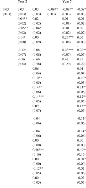
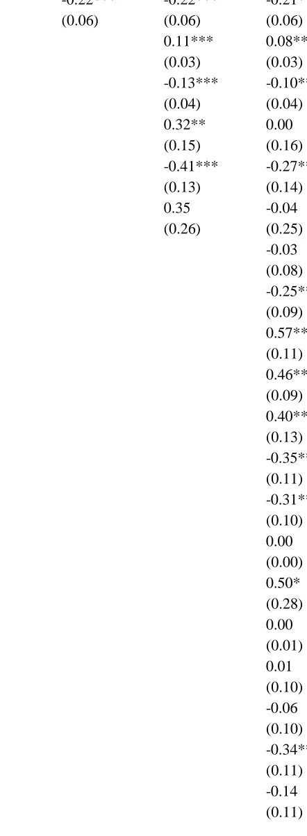
Table A.3 gives in more detail the positive effect on earnings; Tables A.4-A.9 show the

negative effects on life satisfaction, perceived financial situation, running out of money, worry,

trouble with debts, and cash left at the end of the month. As would be expected -- assuming the

randomization had been done effectively -- these tables suggest that there is almost no difference

between the raw estimate of the treatment effect and the estimate after adjustment for people’s

observed characteristics.

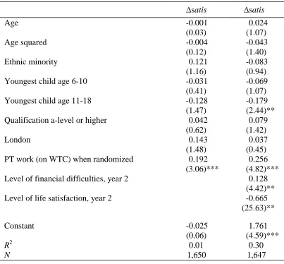
One issue raised in seminar presentations of this work was how different kinds of

individuals within the treatment group fared over the ensuing 5 years. Table B.1 reports data on

this. The dependent variable is the change in life satisfaction. Gainers tend to be those initially

in part-time work (see the first column of Table B.1). Those with higher satisfaction at year 2

saw the greatest fall (column 2 of Table B.1), although some of this may be explicable as simple

mean-reversion.

Some other information is relevant. First, with regard to take-up of the financial bonuses,

these are for those in the treatment group who responded to the 5-year survey. Only those

individuals who worked full-time for sufficiently long could receive the bonus, so non-receipt

cannot be regarded as these individuals ignoring the policy. Approximately 36% received a

bonus. Of those who did, 90% continued after the bonus payments ended to work the same

hours per week as when they were collecting bonuses. Of those who changed their hours after

the bonus payments ended, 19% worked more hours, 44% worked fewer hours, and 37% stopped

working altogether. These percentages are based on just 57 individuals (the 10% who did not

continue to work the same hours). However, among who changed their hours following the end

of the bonus, only 9% reported that this was a direct result of the bonuses ending. Far more

commonly it was due to some other reason.

It is also interesting to consider what might have happened to fertility. The survey does

not capture precise ages of children post-randomization. However, it does ask about the number

of children under 5. Since this is a Year-5 survey (approximately), this could be expected to

capture any effect on additional children as a result of the ERA treatment. In fact, there does not

appear to be any effect. In both the treatment and control groups, 16% of women have a child

under the age of 5. Nor was there any apparent effect on partnering: 22% of women reported

4. Conceptual Issues

One issue for economists and behavioral scientists is how conceptually to make sense of

the main empirical finding of the study. Some possible analytics are set out below. The results

of the randomized trial hold independently of a model, of course, so deductive reasoning is able

only to offer ex post theoretical ideas that will have to be scrutinized in detail in future research

inquiries. Nevertheless, it is perhaps worth speculating on theoretical structures.

Assume that individuals have a utility function which depends on income and the effort

the person puts in at work. Effort is not hours; it is intensity. Assume that the cost of effort, e,

can be summarized by a convex and increasing function c(e). Define net utility, V, as the

difference between the utility from income and the cost of effort. For simplicity, let earned

income be thought of as the product of effort, e, times an earnings piece-rate, p. This is more

general than the traditional assumption of an income-hours trade-off; it allows for the possibility

that people choose high-intensity jobs in return for greater wages.

Non-workers

Assume that some individuals find it optimal not to work. They receive non-labor

income Y. Their effort level, e, is effectively zero. Assume their total income is uncertain, but

that there is a certain (that is, riskless) unemployment-benefit payment, b. Assume that with

probability they also receive -- perhaps in gifts from family or friends or in payment for black

market work they do not declare -- an extra amount of income, y. But assume that with

probability 1- they receive nothing from this source.

Individuals must decide on their consumption spending while bearing in mind their likely

income flows and the uncertainty surrounding those. In total, the expected income of

EY = b + y + (1-  b + y

= c Consumption of non-workers

where c in this equation is defined to be consumption, which is thus assumed set equal to

expected income. This formulation implies that on occasions the individual will run out of

money. More precisely, for those individuals who do not take a paid job, the probability of

running short of cash is 1 – .

Workers

Consider those who take a job. Think of them as earning an amount given by their effort

times the piece rate for that particular job. Like non-workers, assume they get some random

unearned income amount, y. Workers get employment income of pe. Assume also that there is a

government subsidy, s, that is payable to those workers who hold a job and not to those out of

work. This subsidy is temporary. It is positive in the first period and becomes zero in the second

period. Workers get utility from these income flows.

Consider workers as potentially caring not just about their own absolute income but also

as having a reference level of income, r. Assume that -- consciously or subconsciously -- people

compare their earnings to that level. Assume that, in part, workers get utility, in an increasing

and diminishing way, from the gap between what they achieve and this benchmark amount

against which they compare their earnings.

Let utility depend potentially on a convex combination of absolute earnings, pe, and of

earnings relative to the reference level, pe - r. Let the weights on these two be z and 1-z.

Therefore, in the classical textbook case, z would be unity, and people would not compare at all

Here ‘net’ utility can be thought of as being given by the difference between the utility

from money and the costs of effort. Write it

V = v(y + zpe +(1-z) (pe – r) + s) – c(e).

This can be simplified in the following way. Define the weighted reference term (1-z)r as what

might be termed the worker’s ‘aspired’ or comparison income level and denote it a. Then net

utility from the above equation can be rewritten as:

V = v(y + pe – a + s) – c(e)

= utility from earned income - aspiration level + subsidy – costs of effort.

where v(.) is a concave, increasing function that is defined on total income, given by non-labor

income y plus earnings and subsidy, pe + s, less the aspiration level, a. In this case, a

utility-maximizing employee chooses his or her effort level to balance the marginal utility gains from

extra income against the marginal cost of extra effort.

Two forces act to push up the overall aspiration level, a, of earnings. One is if the worker

has a lower z (namely, a lower utility weight on pure absolute earnings, and thus a higher one on

relative pay). The second is if the worker has an intrinsically higher r (namely, a higher base

reference level of income).

Assume utility is defined over two periods (the present and the future) and workers

behave in an optimizing way. Let their effort levels in each period be respectively e and  .

Assume that the piece-rate is defined on the unit interval, so the highest rate that can be earned is

1 and the lowest is zero. It is uncertain ex ante, so p is characterized by a probability density

function f(p). Loosely, high values of the piece-rate p might be thought of as corresponding to a

dp p f c s a p y Ev e c s pe y

Eu( ) ( ) ( ( )) ( )} ( )

{ 1 0         



This form of maximand captures the two periods with two utility functional forms, u(.) and v(.).

Without loss of generality, it normalizes aspiration levels by setting them equal to zero in the

first period. In this specification, there are two random variables because y is random and p is

random. The aspiration level is written a(s) by the assumption that high income subsidies today

could lead to higher aspired income levels in the future.

In this notation, the people who find it desirable not to work are those with low marginal

utility from income. They rely only on non-labor income, so over the two periods their utility is

given by

EU = Eu(y) + Ev(y) A non-worker’s utility

Such individuals face no effort costs.

For those who find it optimal to work, the subsidy s is a non-differentiable function

where above some effort level the amount of s is fixed. This means that workers may be at a

corner where they are minimizing their effort subject to (just) being able to collect the subsidy s.

Initially, however, consider an interior maximum. Then workers choose their effort, in each of

the two periods, to ensure that the first-order conditions for an optimum are

e : { ( ) ( )} ( ) 0

1 0      



:

 { ( ( )) ( )} ( ) 0

1 0      



The more unusual equation is the second. By period 2, in this framework, workers have

developed greater aspirations -- brought on by the higher income that was itself brought on by

people have a higher marginal utility from earned income, because they evaluate their income

flow with respect to the new, and more stringent, aspiration level, a.

We then have the following results.

Proposition 1. Assume a is positive and sufficiently large. Assume that the structure of the

person’s first-period utility function u(.) is exactly, or sufficiently, similar to that of their

second-period utility function v(.). Then:

(i) Workers’ effort levels in the second period are as high as, or higher than, in the first

period e.

(ii)Their utility is lower in the second period than in the first period (and also lower than

the utility of the marginal non-worker).

(iii)Earnings remain high in the second period even though the subsidy has been removed.

(iv)In a significant class of cases, workers run out of money more in the second period

than do non-workers.

The proof of (i), which helps establishes the key element of the other parts of the proposition, is

by contradiction. Assume the reverse, namely, that e . Then, by the convexity of the cost

function,

) ( ) (e c 

c   .

Therefore, rearranging the first-order conditions,

dp p f p s a p y v E dp p f p s pe y u

E ( ) } ( ) { ( ( )) } ( )

{ 1 0 1 0       

_



However, at any given p and y, it must be the case, by concavity of utility, and the fact that s is

positive and a(s) is non-negative, that

)) ( (

)

(y pe s v y p a s

Then, by the monotonicity of the E operator over uncertain y, we can take expectations of both

sides and preserve the inequality sign:

) ( (

)

(y pe s Ev y p a s u

E         ).

Repeating the same step for the piece-rate distribution, by the monotonicity of the expectations

operator it must be that

dp p f p s a p y v E dp p f p s pe y u

E ( ) } ( ) { ( ( )) } ( )

{ 1 0 1 0       

_



But by the first-order conditions this condition can only hold if c(e)c()which in turn

establishes the necessary contradiction.

It might be thought that, as a matter of accounting, all workers would set their

consumption after the actual price p is known, but this framework allows for forward-looking

consumption choices. What happens instead in this framework, therefore, is that those who work

in the second period set their overall consumption level, c*, equal to the expected income level,

so

Consumption of a worker = * [ ( ) ( ) ]

* 0 1 *





c  

where p* plays a particular role explained below.

This formulation does not mean that individuals will never run out of income. They often

will. To see this, it is helpful to define p* as the piece-rate level at which workers just break

even. Below p*, they run short of cash. How often these workers run out of money will depend

upon the covariance between the shocks to non-labor income y and the shocks to piece-rate p.

But it is straightforward to see that there will be a class of cases where the probability of running

is where y is arbitrarily small. Then any p<p* will result in the worker consuming more than is

being earned at that point and hence being short of money.

Loosely, the more right-skewed is the f(.) distribution, the more often will a worker tend

to run out of money. Using Markov’s inequality, the expected piece-rate can be written as







and the greater is f(.) at the upper end of the unit interval the lower must be the value of p*.

Point (ii) in the list earlier implies that v(y + pζ – a(s)) – c(ζ) < v(y + pe) – c(e). The

change in period 2 utility resulting from an ERA-like intervention is then [v(y + pe + pΔ – a(s))

– v(y + pe)] – [c(e + Δ) –c(e)], where Δ = ζ – e. Since utility and cost-functions are increasing,

the first bracketed term is positive if pΔ > a(s) and the second bracketed term is positive. So,

ERA will reduce period 2 utility if individuals do not increase their effort such that earnings go

up at least as much as aspiration income (i.e. pΔ ≤ a(s)). However, we know that, without ERA,

optimizing individuals choose their level of e such that any effort in excess of that level increases

costs more than the positive utility element. It follows then that this also holds with ERA. So,

under ERA, e in that period is set at the rational choice of effort but this is associated with lower

utility than would be the case without ERA.

These results can be put in a more intuitive way. If the government offers a temporary

subsidy to people who take a job, some individuals will respond to that incentive. They will

choose to exert effort and earn more in the first period (that is, the period in which the subsidy

applies) than the individuals who continue not to work. However, in the framework described

here, for the workers who are persuaded into the workforce there is a kind of sting in the tail. If

the first period of earning leads workers to revise up their aspirations, then in the second period

money. There are three consequences. The first is that the employees work hard in the second

period and thus earn income. Their underlying motivation, it might be argued, has been altered:

their greater income aspirations mean that at any income level the marginal utility of earning is

larger than it was before the subsidy scheme. The workers now feel they need extra money.

Because they are less satisfied at each level of income than they were originally, it will be

optimal to work intensively even after the subsidy has been withdrawn. However, all this comes

at the expense of net utility. Workers are eventually less happy, even if earning the same as they

were. In comparison to an individual who was indifferent between taking the subsidized job and

not working, and who ultimately chose the latter, the workers who take the subsidy have lower

utility in the second period than do the non-workers.

This analytical result has the flavor, although not the detail, of prospect theory. Losses

loom larger than gains. Despite the period-1 advantage from taking the government subsidy,

those workers -- who by then are no longer able to draw the subsidy -- have in period 2 to live

with the curse of raised aspirations. Workers thus become richer but not happier.

In the interest of balance, it should be emphasized that the conceptual framework we

develop, while potentially helpful in interpreting the findings of this study, has its own

limitations. A truly general model would allow for the possibility that individuals' cost functions

might also change over time. One of the hopes behind interventions such as ERA is that the

support made available might help people overcome psychological and other barriers to

employment. These barriers contribute to the 'costs' of employment initially but may feature less

prominently once a fuller adjustment to working life has been made. In this scenario, the

results in the current study suggests that any such changes to subjective costs are likely to be of

insufficient size to alter the insights from our simpler model.

5. Checks

Two empirical concerns deserve final consideration.

First, although this study’s RCT is of a well-defined kind, a potentially interesting further

question -- as a matter of statistical description rather than causal inference -- can be asked.

Within the treatment group, who is particularly strongly affected by the intervention? We

examine this in Appendix B.

Second, although in this study we are obliged to deal with the available data, in which

people must voluntarily agree to fill up survey forms (we cannot compel them to do so), a

potential weakness is that there might be selective attrition from the experiment over the ensuing

five years in which we are especially interested. Attrition itself is not, in principle, a problem.

However, differential rates of attrition from the treatment and control groups could be, because

that might lead to biased estimates. On this, Appendix C provides some evidence that -- for our

key finding that the quality of individuals’ lives apparently worsens -- attrition bias is unlikely to

be severe.

6. Conclusions

This paper has examined the outcome of a social-science experiment funded by the

government of the United Kingdom. The study explores the hypothesis that the provision of

temporary in-work benefits will produce an improvement in the quality of people’s lives. Our

results do not support that hypothesis. Methodologically, this inquiry rests on the use of

randomized trials as one standard for reliable empirical knowledge, and it considers as a

their lives more after a policy intervention. With honorable exceptions (such as Ludwig et al.

2012), there have been almost no large RCTs of economic policies in which well-being variables

are taken as the primary outcome criteria.

The purpose of the randomized controlled trial was to discover how labor-market

interventions to help disadvantaged workers might best be designed. The results reveal -- at

least for an important illustrative case -- that traditional ways of making and evaluating labor

market policy can produce striking, and potentially concerning, results. Years after the ERA

randomized intervention finished, those in the treated group were less satisfied with life and

worried more. From a well-being perspective, randomly assigning in-work benefits appears to

have hurt rather than helped. This finding is not what most scholars would have predicted. It is,

however, somewhat reminiscent of the negative results in the Cambridge-Somerville experiment

in the late 1930s, in which disadvantaged boys assigned a mentor, and given other help, went on

to have worse (criminal) outcomes than those in a control group. McCord (1978) suggested that

the intervention in that sample may have created unrealistic expectations in the males in the

treatment group, and that the ultimate effect was thus worse than no intervention. It is possible

that an equivalent mechanism is at work here.

Although it cost multiple millions to fund, the inquiry described here is methodologically

a simple one. One vision of the future of economics is that it develops into an experimental

discipline in which RCTs of this kind become commonplace. In substantive terms, this study

demonstrates the possibility of well-being effects that can run fundamentally counter to intuitive

expectations. Future studies will have to aim to allow society to reach an informed view on

whether, and if so how widely, such findings generalize.

References

M. Adler, E.A. Posner. Happiness research and cost-benefit analysis. Journal of Legal Studies

37, S253-S292 (2008).

K. Baicker, S.L. Taubman, H.L. Allen, et al. The Oregon Experiment: Effects of Medicaid on clinical outcomes. New England Journal of Medicine 368, 1713-1722 (2013).

O. Bargain, K. Orsini. In-work policies in Europe: Killing two birds with one stone? Labour Economics 13, 667-697 (2006).

D.J. Benjamin, O. Heffetz, M.S. Kimball, A. Rees-Jones. What do you think would make you happier? What do you think you would choose? American Economic Review, 102, 2083-2110 (2012).

M. Brewer, M. Francesconi, P. Gregg, et al. In-work benefit reform in a cross-national perspective: Introduction. Economic Journal, 535, F1-F14 (2009).

G. Burtless. The case for randomized field trials in economic and policy research. Journal of Economic Perspectives 9, 63-84 (1995).

G. Burtless. Place randomized trials: Experimental tests of public policy. Journal of Policy Analysis and Management 26, 694-700 (2007).

D. Card, D.R. Hyslop. The dynamic effects of an earnings subsidy for long-term welfare recipients: Evidence from the self sufficiency project applicant experiment. Journal of Econometrics 153, 1-20 (2009).

R. Di Tella, R. MacCulloch, A.J. Oswald. Preferences over inflation and unemployment: Evidence from surveys of happiness. American Economic Review 91, 335-341 (2001).

P. Dolan, R. Metcalfe. Measuring subjective well-being: Recommendations on measures for use by national governments. Journal of Social Policy 41, 409-427 (2012).

R. Dorsett, P.K. Robins. A multi-level analysis of the impacts of services provided by the UK Employment Retention and Advancement Demonstration. Evaluation Review, forthcoming 2014.

E.W. Dunn, L.B. Aknin, M.I. Norton. Spending money on others promotes happiness. Science

319, 1687-1688 (2008).

N. Eissa, H.W. Hoynes. Taxes and the labor market participation of married couples: the earned income tax credit. Journal of Public Economics 88, 1931-1958 (2004).

K. Foley, S. Schwartz. Earnings supplements and job quality among former welfare recipients: Evidence from the self-sufficiency project. Relations Industrielle: Industrial Relations 58, 258-286 (2003).

L.A. Gennetian, C. Miller, J. Smith. Turning welfare into a work support: Six-year impacts on parents and children from the Minnesota Family Investment Program, New York: MDRC. (2005).

H. Gintis. Beyond homo economicus: Evidence from experimental economics. Ecological Economics 35, 311-322 (2000).

C. Graham, M. Nikolova. Does access to information technology make people happier? Insights from well-being surveys from around the world. Journal of Socio-Economics 44 126-139 (2013).

P. Gregg, S. Harkness, S. Smith. Welfare reform and lone parents in the UK. Economic Journal

119, F38-F65 (2009).

G.W. Harrison, List J.A. Field experiments. Journal of Economic Literature 42, 1009-1055 (2004).

L. Haynes, O. Service, B. Goldacre, D. Torgerson. Test, Learn, Adapt: Developing Public Policy with Randomized Controlled Trials. London: Cabinet Office. (2012)

J. Heckman, B. Singer. A method for minimizing the impact of distributional assumptions in econometric models for duration data. Econometrica 52, 271–320 (1984).

R. Hendra, K. Dillman, G. Hamilton et. al. How effective are different approaches aiming to increase employment retention and advancement? Final impacts for twelve models. New York: MDRC. (2010).

R. Hendra, J., Riccio, R, Dorsett, et al. Breaking the low-pay, no-pay cycle: Final evidence from the UK Employment Retention and Advancement (ERA) demonstration Research Report Number 765, Department for Work and Pensions (2011).

J. Helliwell, H.F. Huang. How’s your government? International evidence linking good government and well-being. British Journal of Political Science 38, 595-619 (2008).

A.C. Huston, C. Miller, L. Richburg-Hayes, et. al. New hope for families and children: Five-year results of a program to reduce poverty and reform welfare. New York: MDRC. (2003).

J. Ifcher, H. Zarghamee. Happiness and time preference: The effect of positive affect in a random-assignment experiment. American Economic Review 101, 3109-3129 (2011).

D. Kahneman, A. Tversky. Prospect theory: An analysis of decision under risk, Econometrica, 67, 263-291 (1979).

R. Layard. Happiness and public policy: A challenge to the profession. Economic Journal 116, C24-C33 (2006).

J. List. The behavioralist meets the market: Measuring social preferences and reputation effects in actual transactions. Journal of Political Economy 114, 1-37 (2006).

J. Ludwig, L. Sanbonmatsu, L.A. Gennetian, et al. Neighborhoods, obesity, and diabetes: A randomized social experiment. New England Journal of Medicine 365, 1509-1519 (2011).

J. Ludwig, G.J. Duncan, L.A. Gennetian, et al. Neighborhood effects on the long-term well-being of low-income adults. Science 337, 1505-1510 (2012).

McCord, J. A thirty-year follow-up of treatment effects. Crime And Family: Selected Essays Of Joan McCord. Temple University Press (original published by American Psychological Association in American Psychologist). ISBN9781592135585. (2007(original published in 1978)).

C. Michalopoulos, D. Tattrie, C. Miller, et. al. Making work pay: Final report on the Self-Sufficiency Project for long-term welfare recipients. Social Research and Demonstration Corporation (2002).

S. Oishi, U. Schimmack, E. Diener. Progressive taxation and the subjective well-being of nations. Psychological Science 23, 86-92 (2012).

A.J. Oswald, S. Wu. Objective confirmation of subjective measures of human well-being: Evidence from the USA. Science 327, 576-579 (2010).

A.J. Oswald, E. Proto, D Sgroi. Happiness and productivity. Journal of Labor Economics, forthcoming. (2014)

J. Pencavel. Labor supply of men: A survey. Handbook of Labor Economics (edited by O. Ashenfelter and R. Layard). Amsterdam, North Holland. (1986).

A. Rangarajan, T. Novak. The struggle to sustain employment: The effectiveness of the Post-employment Services Demonstration. Princeton, NJ: Mathematica Policy Research, Inc. (1999).

B. Stevenson, J. Wolfers. Subjective well-being and income: Is there any evidence of satiation?

J. Stiglitz et al. Commission on the Measurement of Economic Performance and Social Progress. September 2009. Downloadable at www.stiglitz-sen-fitoussi.fr.

A.A. Stone, J.E. Schwartz, J.E. Broderick, et al. A snapshot of the age distribution of psychological well-being in the United States. Proceedings of the National Academy of Sciences of the USA 107, 9985-9990 (2010).

R.H. Thaler, H.M. Shefrin. An economic theory of self-control. Journal of Political Economy

89, 392-406 (1981).

APPENDIX A: Design of the Project and Detailed Checks

Details of the evaluation design

The experiment was conducted in 6 regions within the UK. Intake to the experiment began

in October 2003 and continued until April 2005. Three groups of individuals were targeted:

 out of work single parents on welfare (“Income Support” – IS);

 single parents working part-time in low-paid jobs that qualified them for in-work

financial support known as the "Working Tax Credit" (WTC – comparable to the

Earned Income Tax Credit in the US)

 long-term unemployed people on welfare (“Jobseeker’s Allowance” - JSA. A key

difference between IS and JSA is that the former placed no requirement on

recipients to look for work).

Welfare, employment and earnings outcomes for five years after randomization were taken

from administrative records. For the two single parent groups, additional outcomes were

available from surveys carried out approximately two years after random assignment and again

approximately five years after random assignment.

Notes on the sample

The analysis in this paper used data collected from surveys and so is restricted to the two

single parent groups. Furthermore, attention is restricted to mothers (who account for 96 per

cent of single parents in the experiment). The analysis presented in the paper is based on single

mothers responding to both year 2 and year 5 survey interviews. Interviews were attempted with

5,444 single mothers. Of these, 3,212 responded at both year 2 and year 5, an overall response

The official report maintained a distinction at all times between the three target groups

listed above and produced results for men and women combined. The main earnings impacts in

that report were based on outcomes observed in administrative data. This was in order to allow

the full sample of experimental participants to be used rather than the sub-sample of survey

respondents and also to avoid issues of survey attrition. There are definitional differences

between the earnings measures available from administrative sources and those collected through

surveys that reduce comparability across the two sources.

Measures of life satisfaction and perceived financial security

The survey collected information on life satisfaction and a range of aspects of individuals'

perceived financial circumstances. The wording of the questions asked is given below. The first

two questions were asked in both the year 2 and year 5 surveys:

Thinking about all aspects of your life at the moment, how satisfied are you with your life as

a whole. Are you ...

(1) very satisfied,

(2) satisfied,

(3) neither satisfied nor dissatisfied

(4) dissatisfied, or

How difficult would you say your financial situation is at the moment.

Is it...

(1) very difficult,

(2) quite difficult,

(3) neither easy nor difficult,

(4) quite easy,

(5) or very easy?

The other questions were asked only at the year 5 interview:

How often would you say, do you run out of money before the end of the week or the month?

(1) always

(2) most weeks/months

(3) more often than not

(4) sometimes

(5) hardly ever

(6) or never?

(7) spontaneous: don't know/too hard to say/varied too much to say

How often would you say you have been worried about money during the last few weeks?...

(1) almost all the time

(3) only sometimes

(4) never?

Thinking back over the past 12 months, how often would you say you have had trouble with

debts that you found hard to repay?

(1) almost all the time

(2) quite often

(3) only sometimes

(4) never?

How often, would you say, do you have money left over at the end of the week, or if you

budget by the month, at the end of the month?

(1) always

(2) most weeks/months

(3) more often than not

(4) sometimes

(5) hardly ever

(6) or never?

(7) spontaneous: don't know/too hard to say/varied too much to say

Basic descriptives for the outcome variables considered

Where necessary, responses to questions were recoded so that for all variables a higher

was recoded to 1, 4 was recoded to 2, 2 was recoded to 4 and 1 was recoded to 5. With this in

mind, some basic descriptives of the transformed variables are provided in Table A.2.

Detailed estimation results

Tables A.3-A.9 provide the full detail of the key estimation results in the paper. These are

the results relating to the UK excluding London. For each outcome measure three sets of results

are shown. These differ in the covariates included in the regressions: the first specification has

no covariates; the second specification includes only age and ethnicity (as firmly exogenous

variables); the third specification includes a full set of baseline information (still exogenous to

Table A.1 The Characteristics of the Sample Who Were Randomized (percentages)

Great Britain London GB, excl. London

Control Treat Control Treat Control Treat

District (col. %)

Scotland 0.13 0.13 0.15 0.15

North East 0.15 0.15 0.17 0.17

North West 0.11 0.12 0.13 0.13

Wales 0.10 0.11 0.12 0.12

East Midlands 0.38 0.37 0.44 0.42

London 0.12 0.12

Highest qualification (col. %)

A level or higher 0.29 0.28 0.27 0.31 0.30 0.27

O level 0.45 0.47 0.49 0.50 0.44 0.46

Other education qualification 0.10 0.10 0.11 0.07 0.10 0.10

None 0.16 0.16 0.13 0.11 0.17 0.17

Months worked in past 3 years (col. %)

12 or fewer months 0.42 0.41 0.52 0.58 0.41 0.39

13-24 months 0.13 0.11 0.13 0.08 0.13 0.12

25-36 months 0.45 0.47 0.35 0.34 0.46 0.49

Last weekly earnings in year pre-RA

(₤) 69.73 71.50 52.94 63.91 71.95 72.50

(69.08) (70.80) (73.11) (84.86) (68.25) (68.70)

Months on welfare in two years

pre-RA 10.14 9.95 12.79 13.04 9.79 9.54

(10.30) (10.34) (10.67) (10.55) (10.20) (10.24)

Quarter of RA (col. %)

Oct 03-Dec 03 0.02 0.02 0.04 0.04 0.02 0.02

Jan 04-Mar 04 0.24 0.22 0.25 0.24 0.24 0.22

Apr 04-Jun 04 0.18 0.18 0.18 0.19 0.18 0.18

Jul 04-Sep 04 0.21 0.22 0.27 0.27 0.21 0.21

Oct 04-Dec 04 0.26 0.26 0.21 0.22 0.27 0.26

Jan 05-Apr 05 0.09 0.09 0.05 0.03 0.09 0.10

Age 34.77 34.97 35.78 34.87 34.63 34.99

(8.05) (8.11) (7.97) (8.30) (8.06) (8.09)

Age of youngest child (col. %)

less than 6 0.43 0.43 0.40 0.49 0.44 0.42

6-10 0.30 0.29 0.30 0.31 0.30 0.28

11-18 0.27 0.29 0.30 0.19 0.27 0.30

Receiving IS or WTC (col. %)

IS 0.49 0.50 0.69 0.71 0.47 0.47

Ethnic minority status (col. %)

White 0.91 0.90 0.68 0.66 0.93 0.93

Non-white 0.09 0.10 0.32 0.34 0.07 0.07

N 1,603 1,723 187 201 1,416 1,522

Table A.2 Mean, standard deviation and distribution of the well-being measures

Year 2 Year 5

Life satisfaction mean 3.59 3.62

standard deviation 1.04 1.07

Distribution:

- very dissatisfied 4.61% 5.21%

- dissatisfied 12.14% 11.02%

- neither satisfied nor

dissatisfied 19.10% 19.33%

- satisfied 47.80% 45.09%

- very satisfied 16.36% 19.36%

Number of observations 3,320 3,322

Financial situation mean 2.18 2.19

standard deviation 0.92 0.92

Distribution:

- very difficult 26.85% 25.78%

- quite difficult 36.22% 36.90%

- neither easy nor difficult 29.92% 30.57%

- quite easy 6.54% 5.87%

- very easy 0.48% 0.87%

Number of observations 3,319 3,320

Run out of money mean 3.76

standard deviation 1.67

Distribution:

- always 16.07%

- most weeks/months 10.66%

- more often than not 9.64%

- sometimes 25.89%

- hardly ever 20.57%

- never 17.16%

Worry about money mean 2.19

standard deviation 1.00

Distribution:

- almost all the time 32.65%

- quite often 25.46%

- only sometimes 32.56%

- never 9.33%

Number of observations 3,323

Trouble with debts mean 2.19

standard deviation 1.00

Distribution:

- almost all the time 11.36%

- quite often 14.46%

- only sometimes 33.78%

- never 40.40%

Number of observations 3,319

Money left over mean 3.62

standard deviation 1.07

Distribution:

- never 29.91%

- hardly ever 26.98%

- sometimes 24.32%

- more often than not 7.01%

- most weeks/months 5.50%

- always 6.28%

Table A.3 Effect of the ERA treatment on weekly earnings (GB excluding London, years 2 and 5)

Year 2 Year 5

ERA 10.94** 11.86*** 8.99** 9.90* 10.75** 11.22**

(4.38) (4.23) (3.93) (5.30) (5.11) (4.84)

Age 11.52*** 8.36*** 18.68*** 15.27***

(1.70) (1.73) (2.08) (2.08)

Age squared (/100) -11.95*** -10.85*** -21.52*** -19.67***

(2.50) (2.45) (3.02) (2.94)

Age missing 71.84*** 9.17 73.31*** 21.00*

(9.88) (9.28) (12.72) (12.63)

Non-white 0.60 -2.64 22.15 10.73

(9.52) (8.85) (13.93) (13.52)

Ethnicity missing 5.09 -29.77 -3.60 -35.80

(29.30) (32.12) (141.27) (137.93)

Youngest child aged

6-10 3.37 2.80

(5.01) (6.36)

Youngest child aged

11-18 21.16*** 16.89**

(5.65) (7.51)

Highest qual: a-level 48.71*** 74.88***

(6.13) (7.50)

Highest qual: o-level 22.06*** 33.64***

(4.91) (5.92)

Highest qual: other 31.45*** 40.29***

(7.78) (8.81)

Worked <=12 months in past 3

years -11.84* -14.37*

(6.18) (8.61)

Worked 13-24 months in past 3

years -23.03*** -21.14**

(6.35) (8.21)

Weekly earnings in

past year 0.42*** 0.37***

(0.05) (0.06)

Earnings in past year

missing 220.31*** 217.89***

(35.86) (33.88)

Months on welfare

(0.31) (0.43)

District: Scotland -6.38 -8.28

(5.93) (7.63)

District: North East -4.40 -0.20

(5.51) (6.64)

District: North West 8.60 22.94***

(6.78) (8.60)

District: Wales 3.62 -5.02

(7.31) (8.26)

RA in Oct 03-Dec

03 3.25 11.96

(13.28) (18.11)

RA in Jan 04-Mar 04 1.02 40.25***

(10.43) (13.12)

RA in Apr 04-Jun 04 -6.01 45.18***

(12.98) (16.46)

RA in Jul 04-Sep 04 -5.43 22.35

(10.70) (14.06)

RA in Oct 04-Dec

04 0.29 30.80***

(9.14) (11.90)

Month: February 3.44 -23.30**

(8.78) (10.11)

Month: March -12.50 -14.12

(13.89) (17.33)

Month: April 5.93 -17.87

(12.54) (15.34)

Month: May 6.22 -27.27*

(12.56) (15.73)

Month: June 2.92 -32.29***

(10.77) (12.52)

Month: July 1.66 -9.21

(7.53) (9.96)

Month: August 1.67 3.70

(9.05) (13.28)

Month: September -2.24 -13.20

(10.71) (13.64)

Month: October -8.43 -26.79**

(9.18) (11.12)

Month: November -2.89 -9.27

(9.97) (12.57)

Month: December -11.02 -2.55

Receiving WTC -0.06 -2.90

(6.72) (8.95)

_cons 128.29*** -123.16*** -69.90** 151.22*** -228.79*** -201.72***

(3.15) (28.18) (31.50) (3.73) (34.51) (39.08)

N 2833 2833 2833 2842 2842 2842

Table A.4 Effect of the ERA treatment on life satisfaction (GB excluding London, years 2 and 5 – higher score indicates higher life satisfaction)

Year 2 Year 5

ERA 0.04 0.04 0.04 -0.09** -0.08** -0.08**

(0.04) (0.04) (0.04) (0.04) (0.04) (0.04)

Age 0.02 0.02 0.04** 0.02

(0.02) (0.02) (0.02) (0.02)

age squared (/100) -0.04 -0.04 -0.07** -0.05*

(0.02) (0.02) (0.03) (0.03)

Age missing 0.12 -0.05 0.13 -0.07

(0.09) (0.10) (0.09) (0.10)

Non-white -0.25*** -0.23** -0.28*** -0.29***

(0.08) (0.09) (0.09) (0.09)

Ethnicity missing -1.26*** -1.37*** -0.96*** -1.13***

(0.26) (0.29) (0.28) (0.33)

Youngest child aged 6-10 -0.05 -0.07

(0.05) (0.05)

Youngest child aged 11-18 -0.05 -0.13**

(0.06) (0.06)

Highest qual: a-level 0.17** 0.21***

(0.07) (0.07)

Highest qual: o-level 0.14** 0.10*

(0.06) (0.06)

Highest qual: other 0.08 0.10

(0.08) (0.08)

Worked <=12 months in past 3 years -0.08 -0.13**

(0.06) (0.07)

Worked 13-24 months in past 3 years -0.08 -0.16**

(0.06) (0.07)

Weekly earnings in past year 0.00 0.00**

(0.00) (0.00)

Earnings in past year missing 0.33** 0.22

(0.14) (0.20)

Months on welfare in past 2 years 0.00 0.00

(0.00) (0.00)

District: Scotland -0.08 -0.08

(0.06) (0.06)

District: North East -0.07 -0.06

(0.06) (0.06)

(0.07) (0.07)

District: Wales -0.03 -0.19***

(0.07) (0.07)

RA in Oct 03-Dec 03 -0.22 0.21

(0.16) (0.16)

RA in Jan 04-Mar 04 -0.11 0.13

(0.11) (0.11)

RA in Apr 04-Jun 04 -0.19 -0.10

(0.13) (0.14)

RA in Jul 04-Sep 04 -0.20* 0.11

(0.12) (0.12)

RA in Oct 04-Dec 04 -0.12 0.02

(0.10) (0.10)

Month: February -0.07 -0.12

(0.09) (0.09)

Month: March -0.19 -0.31*

(0.14) (0.18)

Month: April 0.02 0.17

(0.12) (0.13)

Month: May 0.02 0.30**

(0.13) (0.14)

Month: June 0.07 0.18*

(0.09) (0.10)

Month: July 0.00 0.09

(0.08) (0.08)

Month: August 0.11 0.05

(0.10) (0.10)

Month: September -0.04 0.02

(0.11) (0.12)

Month: October -0.06 0.02

(0.10) (0.10)

Month: November -0.07 0.02

(0.10) (0.11)

Month: December -0.16 0.06

(0.11) (0.11)

Receiving WTC 0.04 0.16**

(0.07) (0.07)

_cons 3.62*** 3.36*** 3.56*** 3.71*** 3.16*** 3.32***

(0.03) (0.29) (0.34) (0.03) (0.31) (0.35)

N 2837 2837 2837 2841 2841 2841

Table A.5 Effect of the ERA treatment on difficulty of financial situation (GB excluding London, years 2 and 5 – higher score indicates better financial situation)

Year 2 Year 5

ERA 0.03 0.03 0.03 -0.09** -0.08** -0.08**

(0.03) (0.03) (0.03) (0.03) (0.03) (0.03)

Age 0.04** 0.02 0.01 -0.01

(0.02) (0.02) (0.01) (0.02)

age squared (/100) -0.05** -0.04* -0.01 0.00

(0.02) (0.02) (0.02) (0.02)

Age missing 0.14* 0.00 0.25*** 0.06

(0.08) (0.09) (0.08) (0.09)

Non-white -0.12* -0.08

-0.23***

-0.20***

(0.07) (0.08) (0.07) (0.07)

Ethnicity missing -0.56 -0.66 0.42 0.23

(0.54) (0.58) (0.29) (0.29)

Youngest child aged 6-10 0.06 0.01

(0.04) (0.04)

Youngest child aged 11-18 0.10** -0.10*

(0.05) (0.05)

Highest qual: a-level 0.14** 0.21***

(0.06) (0.06)

Highest qual: o-level 0.14*** 0.12**

(0.05) (0.05)

Highest qual: other 0.09 0.15**

(0.07) (0.07)

Worked <=12 months in past 3

years -0.04 -0.11*

(0.06) (0.06)

Worked 13-24 months in past 3

years -0.04 -0.14**

(0.06) (0.06)

Weekly earnings in past year 0.00 0.00

(0.00) (0.00)

Earnings in past year missing 0.46*** 0.40**

(0.16) (0.16)

Months on welfare in past 2 years 0.00 -0.01*

(0.00) (0.00)

District: Scotland -0.12** -0.02

(0.05) (0.06)

District: North East 0.00 -0.02

District: North West -0.08 -0.09

(0.06) (0.06)

District: Wales 0.02 -0.10*

(0.06) (0.06)

RA in Oct 03-Dec 03 0.09 -0.04

(0.13) (0.13)

RA in Jan 04-Mar 04 -0.05 -0.07

(0.10) (0.10)

RA in Apr 04-Jun 04 0.01 0.00

(0.12) (0.12)

RA in Jul 04-Sep 04 0.03 -0.05

(0.10) (0.11)

RA in Oct 04-Dec 04 -0.06 -0.14

(0.09) (0.09)

Month: February -0.10 -0.13

(0.08) (0.08)

Month: March 0.20 0.04

(0.14) (0.14)

Month: April 0.01 -0.11

(0.12) (0.11)

Month: May -0.06 -0.05

(0.11) (0.11)

Month: June 0.00 0.06

(0.09) (0.09)

Month: July -0.02 0.06

(0.07) (0.07)

Month: August -0.15 0.02

(0.09) (0.09)

Month: September -0.11 -0.01

(0.10) (0.10)

Month: October 0.00 -0.01

(0.09) (0.08)

Month: November -0.03 0.04

(0.09) (0.09)

Month: December -0.12 -0.13

(0.10) (0.10)

Receiving WTC 0.16*** 0.00

(0.06) (0.06)

_cons 2.19*** 1.52*** 1.68*** 2.26*** 2.10*** 2.48***

(0.02) (0.28) (0.32) (0.02) (0.26) (0.29)

N 2837 2837 2837 2837 2838 2838

Table A.6 Effect of the ERA treatment on how often money runs out (GB excluding London, year 5 – higher score indicates run out of money less often)

ERA -0.22*** -0.22*** -0.21***

(0.06) (0.06) (0.06)

Age 0.11*** 0.08***

(0.03) (0.03)

age squared (/100) -0.13*** -0.10***

(0.04) (0.04)

Age missing 0.32** 0.00

(0.15) (0.16)

Non-white -0.41*** -0.27**

(0.13) (0.14)

Ethnicity missing 0.35 -0.04

(0.26) (0.25)

Youngest child aged 6-10 -0.03

(0.08)

Youngest child aged 11-18 -0.25***

(0.09)

Highest qual: a-level 0.57***

(0.11)

Highest qual: o-level 0.46***

(0.09)

Highest qual: other 0.40***

(0.13)

Worked <=12 months in past 3 years -0.35***

(0.11)

Worked 13-24 months in past 3 years -0.31***

(0.10)

Weekly earnings in past year 0.00

(0.00)

Earnings in past year missing 0.50*

(0.28)

Months on welfare in past 2 years 0.00

(0.01)

District: Scotland 0.01

(0.10)

District: North East -0.06

(0.10)

District: North West -0.34***

(0.11)

District: Wales -0.14

RA in Oct 03-Dec 03 -0.29 (0.24)

RA in Jan 04-Mar 04 0.08

(0.18)

RA in Apr 04-Jun 04 -0.15

(0.21)

RA in Jul 04-Sep 04 0.04

(0.19)

RA in Oct 04-Dec 04 -0.02

(0.16)

Month: February -0.16

(0.14)

Month: March 0.29

(0.22)

Month: April 0.24

(0.20)

Month: May 0.34*

(0.20)

Month: June 0.05

(0.16)

Month: July 0.14

(0.12)

Month: August 0.13

(0.15)

Month: September -0.15

(0.17)

Month: October -0.05

(0.15)

Month: November -0.04

(0.16)

Month: December -0.08

(0.18)

Receiving WTC 0.01

(0.11)

_cons 3.92*** 1.84*** 2.18***

(0.04) (0.47) (0.52)

N 2831 2831 2831