Constraining bridges between levels of analysis : a computational justification for locally Bayesian learning

warwick.ac.uk/lib-publications

Sanborn, Adam N. and Silva, Ricardo. (2013) Constraining bridges between levels of analysis : a computational justification for locally Bayesian learning. Journal of Mathematical

Psychology, Volume 57 (Number 3-4). pp. 94-106.

Permanent WRAP URL:

http://wrap.warwick.ac.uk/57365

Copyright and reuse:

The Warwick Research Archive Portal (WRAP) makes this work by researchers of the University of Warwick available open access under the following conditions. Copyright © and all moral rights to the version of the paper presented here belong to the individual author(s) and/or other copyright owners. To the extent reasonable and practicable the material made available in WRAP has been checked for eligibility before being made available.

Copies of full items can be used for personal research or study, educational, or not-for-profit purposes without prior permission or charge. Provided that the authors, title and full bibliographic details are credited, a hyperlink and/or URL is given for the original metadata page and the content is not changed in any way.

Publisher’s statement:

© 2013, Elsevier. Licensed under the Creative Commons Attribution-NonCommercial-NoDerivatives 4.0 International http://creativecommons.org/licenses/by-nc-nd/4.0/

A note on versions:

The version presented here may differ from the published version or, version of record, if you wish to cite this item you are advised to consult the publisher’s version. Please see the ‘permanent WRAP URL’ above for details on accessing the published version and note that access may require a subscription.

Constraining Bridges Between Levels of Analysis: A

Computational Justification for Locally Bayesian

Learning

Adam N. Sanborna, Ricardo Silvab

a_{Department of Psychology, University of Warwick} b_{Department of Statistical Science, University College London}

Abstract

demonstrate that a scheme that maximizes computational fidelity while using a restricted factorized representation produces the trial order effects that motivated the development of LBL. This scheme uses the same modular motivation as LBL, passing messages about the attended cues between modules, but does not use the rapid shifts of attention considered key for the LBL approximation. This work il-lustrates a new way of tying together psychological and computational constraints.

Keywords: rational approximations; locally Bayesian learning; trial order effects

Our goal when we model behavior depends on the level of analysis. If we analyze behavior at Marr (1982)’s computational level, then we aim to deter-mine the problem that people are attempting to solve. Or, as more often found in psychology, we might be interested in the mechanism that drives behavior, placing us at Marr (1982)’s algorithmic level. In human and animal learning, both computational-level (Courville et al., 2005; Danks et al., 2003; Dayan et al., 2000) and algorithmic-level models (Rescorla & Wagner, 1972; Mackintosh, 1975; Pearce & Hall, 1980) have been developed. Models developed at different levels of analy-sis have different strengths and this can be seen in how these models of human and animal learning are applied: computational-level approaches are used to explain how organisms are sensitive to complex statistics of the environment (De Houwer & Beckers, 2002; Mitchell et al., 2005; Shanks & Darby, 1998) and algorithmic-level models are used to explain how organisms are sensitive to the presentation order of trials (Chapman, 1991; Hershberger, 1986; Medin & Edelson, 1988).

mod-els that ignore the computational level risk making incorrect or no predictions for task variants (Griffiths & Tenenbaum, 2009; Sanborn et al., 2013). A clas-sic way to combine computational- and algorithmic-level insights is to begin with an algorithmic-level model developed to fit human behavior and then investigate its computational-level properties (Ashby & Alfonso-Reese, 1995; Gigerenzer & Todd, 1999). This is not the only possible direction, and recently researchers have begun at the computational level of analysis and then worked toward understand-ing the algorithm (Griffiths et al., 2012; Sanborn et al., 2010; Shi et al., 2010). Identifying the algorithm to associate with a computational-level model adds both psychological plausibility and explanatory power – computational-level models often are intractable, so the algorithm can provide a computationally tractable approximation while also explaining behavior that differs from predictions of the computational-level model as the result of the approximation. A major open ques-tion is how to select an approximaques-tion algorithm from the vast set of all algo-rithms, and again here human and animal learning provides examples of how this can be done.

from that of the computational-level model it is based upon, Globally Bayesian Learning (GBL). LBL, unlike GBL, is able to successfully predict several effects of trial order on behavior, such as highlighting and the difference between forward and backward blocking. These effects are challenging because there are aspects for which earlier trials have greater influence, known as primacy effects, and as-pects for which later trials have greater influence, known as recency effects, but computational-level models of behavior generally weight all trials equally.

Daw et al. (2008) motivate a bridge between the computational and algorith-mic levels in a different way. Like with LBL, the approximation to the computational-level model is chosen because it reduces computational complexity while pro-viding a better fit to human trial order behavior. However, computational in-stead of psychological considerations are used to select the approximation: A sequential updating algorithm is chosen from those that have been used in com-puter science and statistics to approximate complex probability distributions. The computational-level model is the Kalman filter (Kalman, 1960), which is a gen-eralization of standard associative learning models (Dayan et al., 2000; Dayan & Kakade, 2001; Kruschke, 2008; Sutton, 1992), and it is approximated using Assumed Density Filtering (ADF; Boyen & Koller, 1998), an algorithm for se-quential updating of a probability distribution. ADF approximates the full joint posterior distribution, which can contain dependencies between variables, with a factorized distribution that assumes the variables are independent. By using this and other approximations, the Kalman filter model is able to produce the same trial order effects that LBL does1.

1_{Kalman filters were also used in a later version of the LBL by arranging two Kalman filters in}

Both of the above motivations for bridging the computational and algorith-mic levels have been criticized, each for not providing enough constraints. The restricted messages used by LBL have been criticized for having no specific com-putational justification (Daw et al., 2008), and thus leaving a great deal of freedom in selecting the content of messages and how they are passed between modules. In contrast, Kruschke (2010) argued that choosing an approximation from com-puter science and statistics is not very constraining, as there are a large number of plausible approximations from computer science and statistics that can be used.

Here we take the view that these motivations are not necessarily in conflict and that both psychological and computational motivations can be used to guide development of bridges between levels of analysis. We first describe LBL and review the trial order effects that are difficult for Bayesian models to produce. We then note that LBL constrains computation by assuming that a factorized pos-terior distribution is used to approximate the full pospos-terior distribution on each trial. Using only this computational constraint and a standard measure of distance between probability distributions, we identify the message passing scheme that best approximates the full posterior distribution. This approximation is a form of ADF, the same approximation used to produce some trial order effects in the Kalman filter model. We show that the accumulation of approximation errors from a sequentially factorized representation alone produces these trial order ef-fects, and that the rapid switching of the attended cues in the LBL messages is not necessary. We next give an example of where the predictions of LBL and the se-quentially factorized representation differ. Finally, we discuss the implications for

attention, compare our approach to other approximations to rational models ap-plied to human cognition, and discuss the prospects for integrating computational and psychological motivations.

1. Computational-Level Models of Learning

In human and animal learning studies, the problem that the organism faces is how to use a set of input cues x (e.g., lights or tones presented to an animal) to predict the outcomet (e.g., the food an animal receives). The statistical approach to this prediction problem is to view the relationship between the input cues and outcome as a probability distribution, p(t,x). A full statistical treatment explains the joint probability of outcomes and input cues on a single trial p(t,x), but we take as a starting point models of the conditional distribution p(t|x), which is all that is needed for prediction of the outcome if the input cues are observed.

Computational-level analyses require both a set of possible hypotheses and a probability distribution over these hypotheses that describes the initial beliefs, called the prior distribution. Here the hypotheses are the possible mappings be-tween the input cues and outcomes. There are many possible mappings, but a common choice is to start with outcomes that result from weighted sums of the input cues, as weighted sums are the basis of the classic Rescorla-Wagner (RW; Rescorla & Wagner, 1972) model. A prior distribution is then put over the possible weights, which completes the specification of the computational-level model.

giving a built-in recency effect to the computational-level model because earlier data is less relevant than newer data. However, the Kalman filter model does not have a mechanism to produce primacy effects.

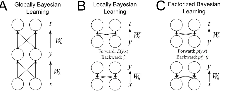
A second approach is GBL (Kruschke, 2006b), which begins with a model that has two levels of weighted sums. A schematic of the model is shown in Figure 1A. Unlike the Kalman filter or RW, GBL includes an early component that determines which input cues to attend to when computing the outcome prediction. The predicted outcome strengthtis a sigmoid function of the weighted sum of the

kattended cuesy,

t=sig(Woy) (1)

whereW_oy is the dot product (element-wise multiplication and then sum) of the

k×1 vector representing the output weights,W_o, and thek×1 vector representing the attended cues,y. The weights were allowed to take discrete values for the sake of simplicity by (Kruschke, 2006b). Each output weight was allowed to take the values of−5, 0, or 5. The weights were combined with the activity of the attention cues and put through Equation 1, and raised to the power of 1.

Likewise, each attended cue’s activation is a sigmoid function of a weighted sum of the input values,

y=sig(W_hx) (2)

whereW_hxis the matrix product between ak×khidden weight matrix,W_h, and a

Each input cue was linked to one attended cue with excitatory weights (in a one-to-one mapping) and linked to every other attended cue with inhibitory weights. As a result of this mapping, each attended cue could be identified with an input cue. To compute the activation of an attended cue, the weights of the present input were summed and put through a sigmoid (i.e., logistic) function as in Equation 2, and raised to the power of 6. This last operation was chosen by Kruschke (2006b) so that activation ranged from nearly zero to nearly one.

Given this specification, the learning done by the model is fixed. Bayes’ rule is used to update the probability distributions over the hidden weights and hidden attentional cues based on the trials that have been experienced

p(Wh,Wo,y|x,t)∝p(t|Wo,y)p(y|Wh,x)p(Wo,Wh). (3)

The prior distribution on the output and hidden weights was independent,

p(W_o,W_h) =p(W_o)p(W_h). The prior p(W_h)was a discrete uniform over all possi-ble combinations of hidden weights. The prior p(W_o)over sets of output weights was set to favor sets of weights that had more values of zero: a product of pseudo-Gaussian distributions2 (φ) with mean zero and standard deviation five for each

weightw_iin the set:∏iφ(wi). Note that this is the prior for the first trial. Through-out this paper we consider the predictions of the model relative to a single trial, rel-egating information from previous trials to the prior to simplify the notation.The prior distribution over weights p(W_h,W_o)is set to the posterior distribution from the previous trial.

2_{The discrete weights were assigned probability proportional to their density under a Gaussian}

GBL learns in a probabilistically correct fashion from experience, but it is a poor fit to the experimental data: unlike the Kalman filter it is necessarily a stationary model and produces neither a primacy nor a recency effect. GBL can also quickly become intractable as the number of input cues grow, as it represents the probability of every combination of possible values of hidden weights and output weights. Forkinput cues andmoutcomes, there are 2k2 possibilities forW_h

and 3kmpossibilities forWo, yielding 2k

2

∗3kmpossibilities for the combinations of

weights. As an illustration of how quickly the number of possibilities grows with the number of input cues, one input cue and one outcome produce six possible combinations of weights, but three input cues and one outcome produces over thirteen thousand weight combinations.

2. Locally Bayesian Learning

Figure 1: Diagrams of Globally Bayesian Learning (GBL), Locally Bayesian Learning (LBL),

and Factorized Bayesian Learning (FBL). Input cues xare weighted by hidden weightsWh and transformed to produce attended cuesy. Attended cuesyare weighted by output weightsWoand transformed to produce outcomest. Multiple outcome nodes are possible as shown here, though only one was required for the tasks we model. The hidden weightsWh, attended cues y, and output weightsWoare not observed and are instead inferred. In GBL, all of the hidden variables are inferred together. LBL splits GBL into two modules with copies of the attended cues yin each module. Messages are passed back and forth between the copies of the attended cues y, the expected valueE(y|x)is passed upward and the single ˆythat maximizes the probability of the outcome is passed backward. FBL uses the same modules as LBL, but the messages passed

between modules are distributions over the attended cues rather than a single set of attended cues.

combinations used in GBL for the same number of input cues and outcomes3. Each LBL module uses Bayes’ rule to update its own representation, but each is prevented from observing the entire state of the environment or the probability distribution represented in the other module. Instead, a module receives some

in-3_{Continuous representations could also be used to reduce the complexity of the hypothesis}

formation indirectly in the form of messages passed from the other module. Mes-sages moving forward from the lower module to the upper contain the expected value of the attended cuesE(y|x). The upper module only observes the expected values of the attended cues and is blind to the input cues. Once the outcome t

has been given, the output weightsWoare updated to be p(Wo|E(y|x),t), instead of the p(W_o|x,t) as they would be in GBL. The expected values of the attended cues given the input are used in the place of the probability distribution over the attended cues given the input.

Messages passed downward from the upper module to the lower module are of a different type. First the output weights are updated, then the value of ythat maximizes the probability of the outcome t is passed downwards to the lower module,

ˆ

y=arg max y∗

∑

p(t|W_o,y∗)p(W_o|E(y|x),t) (4)

The lower module only observes ˆy and the input cues, so the hidden weight prior p(W_h) is updated to be p(W_h|x,yˆ). The restricted messages passed in LBL and the trial-by-trial updating of the representation result in its predictions de-pending on the order of the training trials, which we discuss in the next section.

3. Trial Order Effects

3.1. Highlighting

Because people are sensitive to the statistics of the environment, we expect that the frequencies of different outcomes would play a role in people’s judgments: a higher frequency outcome should produce a stronger relationship than a lower frequency outcome. However, people can display unusual responses to the relative frequency of trials in an experiment, such as the inverse base-rate effect (Gluck & Bower, 1988; Medin & Edelson, 1988). The inverse-base rate effect occurs following two types of training trials. In the first, two input cues, I and Pe, are associated with an outcome E. We will write this asI.Pe→E. The second set of trials pairs one of the old input cues, I, with a new input cue Pl, and a new outcomeL. The labels associated with the input cues and outcomes indicate their roles (which participants must learn from experience): input cueI is an imperfect predictor, input cuePeis a perfect predictor of early outcomeE, and input cuePl

is a perfect predictor of late outcomeL. When given a test trial with input cueIor with conflicting input cues PeandPl, it is reasonable to expect that the response chosen would depend on the relative frequencies of the two types of trials. If there were moreI.Pe→Etrials thanI.Pl→Ltrials, then participants should respondE

given input cueI or the conflicting input cuesPe.Pl. However, Medin & Edelson (1988) found that while participants chose the higher frequency outcome if given input cueI, they chose the lower frequency outcome if given the conflicting input cuesPe.Pl.

inverse base rate effect has been renamed highlighting, the name following from an attentional explanation of the effect. Participants first learn that input cues I

andPeequally predict outcomeE, because they are both equally predictive of the outcome in the I.Pe→E trials. However, the laterI.Pl →L trials demonstrate the ambiguity of input cueI and highlight the relationship between input cuePl

and outcomeL, so participants heavily weight this latter relationship. During test, there is both a primacy effect and a recency effect. The primacy effect is thatIhas a stronger relationship with outcomeE. The recency effect is that if input cuesPe

andPlcompete against each other, outcomeLis chosen becausePlhas a stronger relationship toLthanPehas toE(Kruschke, 1996).

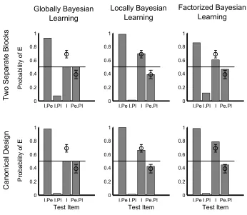
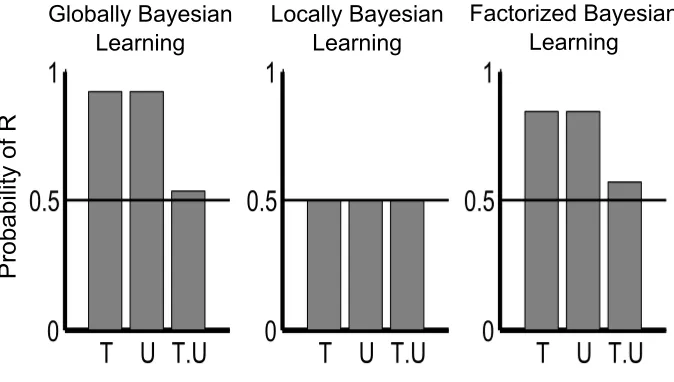
Kruschke (2006a,b) demonstrated that highlighting was an extremely chal-lenging effect for Bayesian models of learning because of the equal number of training trials of each type. The predictions of GBL for two types of highlighting designs are shown in Figure 2. The first design was used in Kruschke (2006b) to demonstrate the models: seven trials of I.Pe →E followed by seven trials of

I.Pl→L. The second design follows more closely that used in Kruschke (2009, design given in the Appendix), in which the human data showed a strong high-lighting effect.

Unlike GBL, the restricted nature of the messages in LBL causes it to pre-dict a robust highlighting effect that matches human data, as shown in Figure 2. The prediction of highlighting was explained by attention to cues to that rapidly switched between trial types, like in the description of highlighting above. The message passed backward from the upper module to the lower module consisted of attended cuesI0andPe0in the early trials4, soI0is activated on these trials and

one-is thus associated with E. However on the second block of I.Pl→Ltrials, as I

already strongly activates E, the attended cue that is maximally consistent with the output weights is Pl0alone soI0is not activated. As a result, Imore strongly activates E and Pl more strongly activates L thanPe activates E, producing the highlighting effect (Kruschke, 2006b).

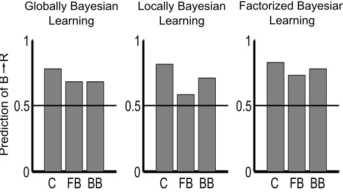
3.2. Forward and Backward Blocking

The experimental effect of blocking demonstrates how input cues compete with each other during learning (Kamin, 1968). As a comparison, control trials consist of two input cues and a outcome, A.B→R, and participants believe that

BpredictsRwith some moderate strength. Forward blocking occurs if this set of training trials is preceded by a set of training trials in which A→R. The initial learning of A→Rblocks the establishment of a relationship of B with Rin the

A.B→Rtrials, asAby itself was sufficient to predict the outcome. After the two blocks of learning, participants believe thatBpredictsRonly weakly.

Forward blocking is a straightforward prediction of RW, but a slight change to the design complicates associative explanations. In backward blocking, the order of the blocks is reversed so that the A.B→Rtrials occur before theA→R

trials. Here the prediction of Rfrom Bis also reduced, though this effect is not as larger or as robust as forward blocking (Beckers et al., 2005; Chapman, 1991; Kruschke & Blair, 2000; Lovibond et al., 2003; Melchers et al., 2006; Shanks, 1985; Vandorpe et al., 2007). Essentially, participants retrospectively re-evaluate the strength of the relationship between BandR, reducing it because of the later

to-one mapping of positive weights between input cues to attended cues. All other weights were

A→Rtrials. Backward blocking is not predicted by RW and so has been taken as evidence for statistical accounts of learning, though modified associative accounts are able to predict it (Van Hamme & Wasserman, 1994).

Backward blocking can be explained by Bayesian models of learning (Gopnik et al., 2004; Sobel et al., 2004; Tenenbaum & Griffiths, 2003), but a difference in strength between forward and backward blocking presents difficulties for many Bayesian models because the two designs differ only in the order of presentation of the training trials (but see Daw et al., 2008; Dayan & Kakade, 2001). Many experiments have shown a trace of this effect (Chapman, 1991; Kruschke & Blair, 2000), and it was shown to be statistically reliable in (Vandorpe et al., 2007). The difference in the size of the effects in this study was found to be between 10% and 20% of the range of the scale.

ignore B. This results in a weak relationship between B and R, asB is ignored during trials in which the relationship could be strengthened. In contrast, in back-ward blocking the maximally consistent message passed from the upper module to the lower module in the first block of backward blocking is to attend to both input cues, strengthening the relationship during this block of training trials. As a result, for LBL,BpredictsRmore strongly in backward than forward blocking.

4. Message Passing and Factorized Representations

The match between LBL and human trial order effects is due to a message passing scheme that was chosen on an ad-hoc basis. There are many possible schemes for passing messages between modules, varying in aspects such as which content is passed, in which sequence and at which loss of information. Despite the multiplicity of possible mechanisms, we argue that there are some general principles that can strongly constrain the possible algorithmic constructions for a computational model. In this section, we initially discuss how the message passing scheme of LBL approximates GBL. We then set the stage to introduce an alternative based on a more fundamental set of algorithmic principles, with the goal of largely retaining the predictive power of LBL without seemingly ad-hoc combinations of approximations.

To understand the design choices behind LBL, let us first summarize how GBL works. For GBL, the posterior distribution over the weights, p(Wo,Wh|x,t), does not factorize into independent contributions from each of the weights, as in

p(Wo|x,t)p(Wh|x,t). Instead,

p(Wo,Wh|x,t) =

∑

GBL has a distribution over the possible attended cues, y, and this range of possibilities means that the posterior distribution does not factorize. A non-factorized distribution requires more memory to represent, and complicates up-dates when new data points are observed. However, we can see in Equation 5 what would happen if y were fixed at a single value: the summation would dis-appear and the posterior distribution would factorize. Exploiting this fact, the representation learned by LBL has the following structure:

1. Consider collapsing our uncertainty over y using an estimate ˜y, which is assumed to be known with certainty (i.e., p(y˜|x,t) =1)

2. To further simplify computation, do not construct a representation with the structure p(W_o,W_h|x,t)≈ p(W_o|y˜,t)p(W_h|y˜,x): instead, use two different estimates where p(Wo,Wh|x,t)≈ p(Wo|y˜1,t)p(Wh|y˜2,x). This means

com-putation can be carried separately within two different modules, one for each factor

3. Under this formulation, use one estimate ˜y_igenerated within one module to compute the other estimate ˜y_j

Within the choices provides by this framework, LBL can be thought as hav-ing a shav-ingle hypothesis, though different in the upwards and downwards mes-sages, passed between modules. LBL’s posterior distribution of p(Wo,Wh|x,t) is a factorized distribution and can be written as the product of the individual weight distributions p(Wo|E(y|x),t)p(Wh|yˆ,x). LBL starts with a factorized prior

Approximations that sequentially factorize the posterior distribution after each data point have been explored in computer science and statistics. This class of approximations is known as Assumed Density Filtering (ADF; Boyen & Koller, 1998). In ADF, the posterior distribution over parameters is approximated with a simpler distribution after each new data point is observed. This approximate posterior is used as the prior when processing the next point.

While LBL’s message passing scheme falls within the class of ADF algo-rithms, there is still the question of whether LBL is a good approximation to the full posterior distribution. We can test LBL’s message passing scheme by examining it within Minka (2005)’s unified framework for generating approxi-mations, which encompasses and generalizes several techniques from machine learning, statistics, statistical physics, and information theory. One key aspect of this framework is that the choice of approximation is based on picking the ap-proximation that is “closest” to p(W_o,W_h |t,x) according to some definition of similarity between probability functions.

Although this similarity-maximization (or, analogously, divergence-minimization) principle might sound too broad, LBL does not seem to obey it. Namely, we have been unable to find any divergence measureD(p,q)where, forp=p(W_o,W_h|t,x)

qo(Wo)qh(Wh), find the one that is closest to the true posterior p(Wo,Wh |x,t)≡

p_x,t(Wo,Wh). We term this approach Factorized Bayesian Learning (FBL) and a schematic of this model is shown in Figure 1C.

Our choice of a message passing scheme depends on our measure of diver-gence. We propose that the choice of q should be the one that minimizes the

Kullback-Leibler(KL) divergence. KL divergence is a popular criterion for choos-ing approximations, since KL(p || q) =0 if and only if p= q, and is positive otherwise (Minka, 2001). It has a long history in information theory (Cover & Thomas, 1991), and has an interpretation based on coding: if a string/sample is generated from distribution p, but encoded using a scheme based on q, the KL divergence is how many extra bits (or nats in our case, because we use base e) are needed to encode the message relative to the optimal code based on p. KL divergence can be written as

KL(p||q) =

Z Z

p(Wo,Wh|x,t)ln

p(Wo,Wh|x,t)

q_o(W_o)q_h(W_h)dWodWh (6)

where the target approximation q(W_o,W_h) takes the shape q_o(W_o)q_h(W_h). The distribution over hidden attended cues yis implicit, since the problem of choos-ingq_o(W_o)q_h(W_h) to minimize Equation 6 is equivalent to choosing the one that minimizes

−

Z Z Z

p(W_o,W_h,y|x,t)ln[q_o(W_o)q_h(W_h)]dW_odW_hdy (7)

Minimizing Equation 6 with respect to q_o(·) and q_h(·) results in q_o(W_o) =

can be rewritten as

−

_∑

Wo

p(W_o|x,t)lnq_o(W_o)−

_∑

Wh

p(W_h|x,t)lnq_h(W_h) (8)

We have to optimize this function with respect to the entries of q_o(W_o) and

q_h(W_h)such that such entries are non-negative and∑Woqo(Wo) =1,∑Whqh(Wh) =

1. Using Lagrange multipliers for this constrained optimization problem and ig-noring for now the non-negativity constraints, this gives the following objective function:

−

_∑

Wo

p(W_o|x,t)lnq_o(W_o)−

_∑

Wh

p(W_h|x,t)lnq_h(W_h)+λo(

∑

q_o(W_o)−1)+λh(

∑

q_h(W_h)−1)

(9) Taking the derivative of Equation 9 with respect to an arbitrary entryq_o(W_o), we obtain

−p(Wo|x,t)/qo(Wo) +λo=0 (10)

which impliesqo(Wo)∝p(Wo |x,t)for all valuesWo. Because ∑Woqo(Wo) =1,

it follows that q_o(W_o) = p(W_o | x,t). The reasoning is analogous when deriving

q_h(W_h) = p(W_h|x,t).

The role of message-passing and prior factorization have algorithmic implica-tions due to the calculation of the marginals. For the output weights,

p(W_o|x,t) ∝ ∑Wh∑yp(t|Wo,y)p(y|Wh,x)p(Wo)p(Wh)

= p(Wo)∑yp(t |Wo,y)∑Wh p(y|Wh,x)p(Wh)

≡ p(W_o)∑yp(t |Wo,y)mx(y)

wherem_x(y)≡∑Whp(y|Wh,x)p(Wh)is the message passed from the lower

x for a given value of y. It is possible to decouple this module from the output module only because the prior overW_oandW_hfactorizes as p(W_o)p(W_h).

Analogously,

p(W_h|x,t) ∝ ∑Wo∑yp(t|Wo,y)p(y|Wh,x)p(Wo)p(Wh)

= p(W_h)∑yp(y|Wh,x)∑Wop(t |Wo,y)p(Wo)

≡ p(W_h)∑yp(y|Wh,x)mt(y)

wherem_t(y)≡∑Wop(t|Wo,y)p(Wo)is the message passed from the upper module

to the lower module that encapsulates all the information content provided bytfor a given value ofy.

5. Factorized Representations for Trial Order Effects

Surprisingly, Figure 2 shows that FBL produces the highlighting effect for the design in Kruschke (2006b) and that the size of the effect matches human data if the model is trained with the same number of stimuli that participants were. Figure 3 shows that FBL also produces the trial order effect for blocking. The FBL highlighting effect and the FBL blocking effect can be better matched to the size in the human data by adjusting the parameters of the model5, but we used the original parameters to demonstrate that the FBL produces the same qualitative effects as LBL with the same parameters. Instead of an explanation that is due to passing the maximally consistent message backwards, this effect is due to the more basic separation of GBL into two modules and the sequential approximation of trials that then results.

Effects of approximation have a long history in comparisons of the most gen-eral artificial algorithmic system, the digital computer, against abstract compu-tational models such as the Turing machine. The field of numerical analysis, in particular, tackles the issue on how problems of mathematical analysis can be solved in practice, considering the accumulation of errors due to the sequential processing of numerical operations using a digital representation. One can, for instance, analyze the computational complexity of a procedure for matrix inver-sion (Cormen et al., 2009), but its numerical stability depends upon the control

5_{Changing the parameters to fit highlighting data must be done carefully. For some parameter}

settings, the GBL does predict a highlighting effect because the critical test items I and Pe.Pl

consist of different numbers of cues, and inhibition only occurs if more than one cue is presented.

of rounding errors that accumulates as the sequence of steps in the algorithm is followed. ADF, and in particular FBL, uses an approximation as input to the next approximation. As the literature of numerical analysis shows us, a combination of biases and sequential processing might lead to results that do not match what the computational model entails.

ADF gives the best approximation with respect to a given prior. However, since in a sequential update scheme the “prior” represents compiled evidence of previous observations, errors will propagate. Minka (2001) suggests, for instance, that ADF is particularly prone to bad approximations of marginals if the input sequence of data points differs considerably from what it should be obtained by a randomized sequence. Hence, FBL dispenses with the necessity of a Kalman filter formulation, since an ordering effect is automatically accounted for by ap-proximation errors.

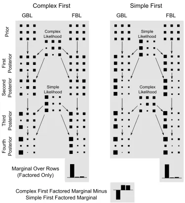
An example that will prove useful for explaining both the highlighting and blocking predictions is shown in Figure 5. GBL and FBL both begin with the same prior distribution and are updated with either data that produce “complex” likelihoods or data that produce “simple” likelihoods. The weights are dependent in the complex likelihood, but independent in the simple likelihood. If FBL and GBL are updated with a simple likelihood, they produce the same posterior distri-butions, as can be seen in the first and second posterior distributions if the simple likelihood is presented first. However, when GBL and FBL are updated with a complex likelihood, their joint posterior distributions diverge.

distributions diverging. The final marginal distributions depend on whether FBL is updated with the two simple likelihoods first or updated with the two complex likelihoods first. The difference between the final marginal distributions (shown at the bottom of Figure 5) is small for such a small number of training trials, but the most likely value is smaller and the other values larger if the complex likelihoods are presented first compared to if the simple likelihoods are presented first. As we explain below, this is what drives both the highlighting and blocking effects. Unlike in the LBL, the trial order effects do not arise from the rapid nature of changes to which cues are attended to, but instead follow directly from computa-tional considerations.

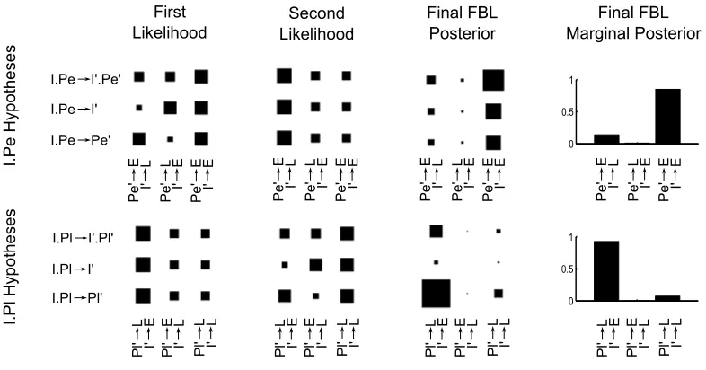
5.1. Predicting Highlighting

The likelihoods for the first and second set of training trials have the same structure as those we used as examples in Figure 5. I.Pe→E trials are presented first, so the first seven likelihoods for I and Pe in the first row of the plot are complex, where if onlyI is attended (activating its corresponding attended cueI0) then both hypotheses in whichI0→Eare more likely than the hypothesis in which

I0→L. Likewise, if onlyPe is attended, then both hypotheses in whichPe0→E

are more likely than the hypothesis in whichPe0→L. However, theI.Pe→Etrials tell us nothing aboutPl. So for the first likelihood of theI.Plhypotheses, we learn thatI0→Eis more likely thanI0→L, but it has no interactions with the attended cues, a likelihood which is simple. The second seven likelihoods are exactly the reverse. TheI.Pl→Ltraining trials gives us a likelihood that is complex between hidden and output weights forI.Plhypotheses, but is simple forI.Pehypotheses. This gives us the same orderings of simple and complex likelihoods as in Figure 5. As a result, we find the same effect on the marginal distributions that we found in Figure 5. When the complex likelihood is first, then the first column is reduced and the third column is boosted compared to when the simple likelihood is first. We can see the highlighting prediction arise from this difference in the marginals6. The combined marginal in whichI0→E are greater than the combined marginals in whichI0→L, giving the prediction for the irrelevant input cue. ForPe.Pl, the combined marginals in which Pe0 →E are less than the combined marginals in whichPl0→L, giving the prediction ofPe.Pl→L.

6_{We ignore the hidden weights here because the test input cueIalone means that there is no}

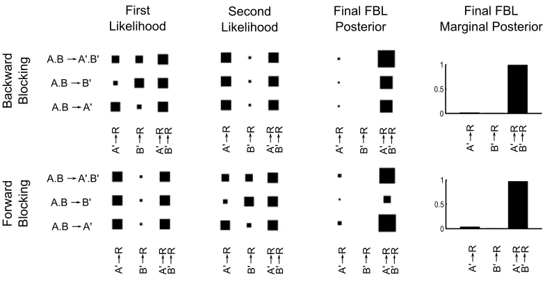
5.2. Predicting Blocking

FBL predicts a difference in strength between forward and backward block-ing for the same reason: the orderblock-ing of complex and simple likelihoods. Figure 7 summarizes the hypothesis space for FBL for blocking. Again, the vertical dimen-sion of each plot shows possible hypotheses about the hidden weights, grouping those hypotheses that do and do not result in the attended cues exceeding an arbi-trary threshold of 0.5 in activation. The horizontal axis groups the output weights by showing the probability of the largest weight and smallest weight for reward. The two rows separately summarize backward and forward blocking. Hypotheses about indifference in output weights are not included in this figure.

Like highlighting, the likelihoods for blocking are either complex or sim-ple, though here the complex or simple likelihoods apply to the entire hypothesis space. In backward blocking the first set of trials areA.B→R, so the combinations of hypotheses that lead to a greater prediction of Rare given greater likelihood. This leads to a dependence between hidden and output weights because if onlyA0

is activated, thenA0→Ris more likely thanB0→R, and the relative ordering of the probabilities reverses ifB0is activated. In forward blocking the first likelihood is simple. We are only learning about A with A→R trials, so we do not learn anything about which cues should be attended.

6. Differences Between Locally Bayesian Learning and Factorized Bayesian

Learning

We have shown FBL is a more principled approximation than LBL and here we demonstrate how the more principled approximation can lead to different pre-dictions. The example we use is a classic in both the artificial intelligence and the human and animal learning literatures: the exclusive-OR (XOR) problem for which the learner is trained to respond to cues singly but not in combination. XOR is a simple version of a nonlinearly separable problem that cannot be learned by a single layer linear network (Minsky & Papert, 1969), but has been shown to be learnable by both animals and humans (also known as negative patterning; Pavlov, 1927; Harris & Livesey, 2008; Harris et al., 2008; Rescorla, 1972, 1973).

Of course a common way to attempt to account for XOR problems is to in-troduce configural units (Minsky & Papert, 1969; Spence, 1952), and indeed Kr-uschke (2006b) proposed this solution for LBL. There is some evidence that con-figural units make the wrong sort of predictions for human and animal behav-ior (Harris & Livesey, 2008; Harris et al., 2008), but if we allow them then this demonstration serves to illustrate a difference between FBL and LBL that could be potentially tested in experiments with more complex XOR designs.

7. Discussion

We have shown how a computationally justified version of LBL can be used to produce human-like trial order effects, and additionally how the FBL potentially better matches human behavior in XOR tasks. Here we investigate the implica-tions for rapid shifts of attention, relate the approximation used in FBL to other approximations hypothesized to be in use in the mind, discuss the hypothesis that modularity corresponds to factorization, and conclude.

7.1. Implications for Rapid Shifts of Attention

needed to be complex (as discussed below) to produce the blocking results as well (Daw et al., 2008).

The current results go beyond these to demonstrate that even in the two layer network of the LBL, in which the output is based on attended cues rather than the observed cues, rapid shifts of attention are not necessary to predict highlighting or the difference between forward and backward blocking. Instead, FBL predicts these results using only the factorization of the probability distributions over the layers of the weights of the network. The message passed backwards from the upper module to the lower module is not a maximization message, but is instead the actual marginal distribution of the attended cues given the outcome of the trial. This indicates that the separation between the modules imposed by the factoriza-tion is sufficient to produce these trial order effects, and that the particular kinds of messages associated with rapid shifts of attention are not necessary.

7.2. Kinds of Approximations

poste-rior produces both the highlighting effect and the difference in strength between forward and backward blocking. For the Kalman filter, factorizing the posterior distribution produces highlighting, but causes backward blocking to disappear. In order to produce both effects, interpolations were made between the sequentially factorized posterior distribution that produces highlighting and the full posterior distribution that produces backward blocking.

The effectiveness of LBL, FBL, and the Kalman filter approximations in trial order effects has wider implications for how we attempt to build bridges between computational- and algorithmic-level analyses. Other research has used sam-pling algorithms from computer science and statistics to bridge computational-and algorithmic-level analyses. This has been done in wide variety of areas, such as categorization (Sanborn et al., 2010; Shi et al., 2010), sentence parsing (Levy et al., 2009), prediction (Brown & Steyvers, 2009), perceptual bistability (Ger-shman et al., 2012), and even human and animal learning (Lu et al., 2008; Ro-jas, 2010) to explain trial order effects. Sampling algorithms tend to come with asymptotic guarantees: with enough samples any computation done with these algorithms will be indistinguishable from computation done with the full proba-bility distribution. To allow for computational tractaproba-bility and to produce devia-tions from the computational-level model, far fewer samples are used. While in some situations we can choose among sampling algorithms to best approximate the posterior distribution (e.g., Fearnhead, 1998) and the number of samples that best balances reward with opportunity cost can at times be computed (Vul et al., 2009), the quality of approximation given by a sampling algorithm is generally not made explicit.

all examples of sequential variational approximations. Instead of representing the distribution with a series of points chosen stochastically from the true distribution, variational approximations are deterministic and approximate a target distribution by choosing a more tractable distribution as a stand in. In terms of trying to fit to human data, variational approximations have the advantage of introducing biases that can be explicitly justified by a divergence measure from the true distribution given particular computational constraints. This opens up a new set of algorithms that can be used for developing rational process models.

7.3. Factorization and Modularity

LBL and FBL both cast modules as factorized probability distributions that are coordinated by statistically-motivated message passing – resulting in central modules with extraordinary flexibility. Other computational approaches have ei-ther worked out how to co-ordinate the output of peripheral modules (B¨ulthoff & Yuille, 1996) or cast modules as complete central procedures that are context-dependent (Jacobs et al., 1991). Here we have introduced modularity that results from sequential co-ordination of modules, and the use of message passing opens up ideas for much more active and principled co-ordination between modules.

One interesting case of modularity is the case where factorization does no harm: when the information is actually independent given the interpretation. For example, participants could be given visual and auditory information in order to estimate an object’s location. Here factorization does not result in the loss of information because these sources are assumed to be independent. Interestingly, participants in this task take into account information about the variability of the cues, and give more weight to cues that are more reliable (Alais & Burr, 2004; Ernst & Banks, 2002). This sort of result is more congruent with FBL than LBL, because FBL passes along an entire distribution over outputs while LBL only passes along the mean of a distribution without information about its variability.

7.4. Conclusions

predic-tions for other experimental designs. Connecpredic-tions between existing models and machine learning algorithms give cognitive scientists access to a rich resource for developing alternative models that produce a range of behavior. Aside from psychological and computational constraints, an exciting prospect is that other constraints can be introduced by neural considerations. The approximations used in the brain are still a new area of investigation, though some work has been done on explaining neural activity using both variational (Friston, 2010; Gershman & Wilson, 2010) and sampling explanations (Fiser et al., 2010). By constraining our search it is hoped that the approximations used in the mind can be identified.

The authors thank John Kruschke, Stephen Denton, Peter Dayan, and David Shanks for helpful discussions.

Alais, D., & Burr, D. (2004). The ventriloquist effect results from near-optimal bimodal integration. Current Biology,14, 257–262.

Ashby, F. G., & Alfonso-Reese, L. A. (1995). Categorization as probability den-sity estimation. Journal of Mathematical Psychology,39, 216–233.

Bechtel, W. (2003). Modules, brain parts, and evolutionary psychology. In S. J. Scher, & F. Rauscher (Eds.),Evolutionary Psychology: Alternative Approaches

(pp. 211–227). Norwell, MA: Kluwer Academic Publishers.

Beckers, T., De Houwer, J., Pineo, O., & Miller, R. R. (2005). Outcome additivity and outcome maximality influence cue competition in human causal learning.

Journal of Experimental Psychology: Learning, Memory, and Cognition, 31, 238–249.

pro-cesses. InProceedings of the Fourteenth Conference on Uncertainty in Artificial Intelligence(pp. 33–42).

Brown, S. D., & Steyvers, M. (2009). Detecting and predicting changes.Cognitive Psychology,58, 49–67.

B¨ulthoff, H. H., & Yuille, A. L. (1996). A Bayesian framework for the integration of visual modules. In T. Inui, & J. L. McClelland (Eds.), Attention and Per-formance 16: Information Integration in Perception and Communication (pp. 49–70). Cambridge, MA: MIT Press.

Carruthers, P. (2006). The Architecture of the Mind. Oxford: Oxford University Press.

Chapman, G. B. (1991). Trial order affects cue interaction in contingency judg-ment.Journal of Experimental Psychology: Learning, Memory, and Cognition,

17, 837–854.

Collins, E. C., Percy, E. J., Smith, E. R., & Kruschke, J. K. (2011). Integrating advice and experience: learning and decision making with social and nonsocial cues. Journal of Personality and Social Psychology,100, 967–982.

Cormen, T. H., Leiserson, C. E., Rivest, R. L., & Stein, C. (2009). Introduction to Algorithms. MIT Press.

Courville, A. C., Daw, N. D., & Touretzky, D. S. (2005). Similarity and discrimi-nation in classical conditioning: A latent variable account. In L. Saul, Y. Weiss, & L. Bottou (Eds.), Advances in Neural Information Processing Systems 17. Cambridge, MA: MIT Press.

Cover, T., & Thomas, J. (1991). Elements of information theory. New York: Wiley.

Danks, D., Griffiths, T. L., & Tenenbaum, J. B. (2003). Dynamical causal learning. In S. Becker, S. Thrun, & K. Obermayer (Eds.), Advances in Neural Informa-tion Processing Systems 15. MIT Press.

Daw, N. D., Courville, A. C., & Dayan, P. (2008). Semi-rational models of con-ditioning: the case of trial order. In N. Chater, & M. Oaksford (Eds.), The Probabilistic Mind(pp. 431–452). Oxford, UK: Oxford University Press.

Dayan, P., & Kakade, S. (2001). Explaining away in weight space. InAdvances in Neural Information Processing Systems.

Dayan, P., Kakade, S., & Montague, P. R. (2000). Learning and selective attention.

Nature Neuroscience,3, 1218–1223.

De Houwer, J. D., & Beckers, T. (2002). Second-order backward blocking and unovershadowing in human causal learning. Experimental Psychology,49, 27– 33.

Fearnhead, P. (1998). Sequential Monte Carlo methods in filter theory. Ph.D. thesis University of Oxford.

Fiser, J., Berkes, P., Orb´an, G., & Lengyel, M. (2010). Statistically optimal per-ception and learning: from behavior to neural representations. Trends in Cog-nitive Sciences,14, 119–130.

Fodor, J. A. (1983). The Modularity of the Mind. Cambridge, MA: MIT Press.

Friston, K. (2010). The free-energy principle: a unified brain theory? Nature Reviews Neuroscience,11, 127–138.

Gershman, S. J., Vul, E., & Tenenbaum, J. B. (2012). Multistability and perceptual inference. Neural Computation,24, 1–24.

Gershman, S. J., & Wilson, R. (2010). The neural costs of optimal control. In J. Lafferty, C. K. I. Williams, J. Shawe-Taylor, R. Zemel, & A. Culotta (Eds.),

Advances in Neural Information Processing Systems 23(pp. 712–720).

Gigerenzer, G., & Todd, P. M. (1999). Simple heuristics that make us smart. Oxford: Oxford University Press.

Gluck, M. A., & Bower, G. H. (1988). From conditioning to category learning: an adaptive network model. Journal of Experimental Psychology: General, 117, 227–247.

Griffiths, T. L., & Tenenbaum, J. B. (2009). Theory-based causal induction. Psy-chological Review,116, 661–716.

Griffiths, T. L., Vul, E., & Sanborn, A. N. (2012). Bridging levels of analysis for probabilistic models of cognition.Current Directions in Psychological Science,

21, 263–268.

Harris, J. A., & Livesey, E. J. (2008). Comparing patterning and biconditional discriminations in humans. Journal of Experimental Psychology: Animal Be-havior Processes,34, 144–154.

Harris, J. A., Livesey, E. J., Gharaei, S., & Westbrook, R. F. (2008). Negative pat-terning is easier than a biconditional discrimination. Journal of Experimental Psychology: Animal Behavior Processes,34, 494–500.

Hershberger, W. A. (1986). An approach through the looking-glass. Learning & Behavior,14, 443451.

Jacobs, R. A., Jordan, M. I., & Barto, A. G. (1991). Task decomposition through competition in a modular connectionist architecture: The what and where vision tasks. Cognitive Science,15, 219–250.

Kalman, R. (1960). A new approach to linear filtering and prediction problems.

Transactions of the ASME – Journal of Basic Engineering,82, 35–45.

Kruschke, J. K. (1996). Base rates in category learning. Journal of Experimental Psychology: Learning, Memory, and Cognition,22, 3–26.

Kruschke, J. K. (2001a). The inverse base-rate effect is not explained by elimi-native inference.Journal of Experimental Psychology: Learning, Memory, and Cognition,27, 1385–1400.

Kruschke, J. K. (2001b). Toward a unified model of attention in associative learn-ing. Journal of Mathematical Psychology,45, 812–863.

Kruschke, J. K. (2006a). Locally Bayesian learning. In R. Sun (Ed.),Proceedings of the 28th Annual Meeting of the Cognitive Science Society (pp. 453–458). Hillsdale, NJ: Erlbaum.

Kruschke, J. K. (2006b). Locally Bayesian learning with applications to retro-spective revaluation and highlighting. Psychological Review,113, 677–699.

Kruschke, J. K. (2008). Bayesian approaches to associative learning: From pas-sive to active learning. Learning & Behavior,36, 210–226.

Kruschke, J. K. (2009). Highlighting: A canonical experiment. In B. Ross (Ed.),

The Psychology of Learning and Motivation(pp. 153–185). volume 51.

Kruschke, J. K. (2010). What to believe: Bayesian methods for data analysis.

Trends in Cognitive Sciences,14, 293–300.

Kruschke, J. K., & Blair, N. J. (2000). Blocking and backward blocking involve learned inattention. Psychonomic Bulletin & Review,7, 636–645.

& M. E. L. Pelley (Eds.), Attention and Associative Learning: From Brain to Behaviour(pp. 273–304). Oxford, UK: Oxford University Press.

Kruschke, J. K., Kappenman, E. S., & Hetrick, W. P. (2005). Eye gaze and in-dividual differences consistent with learned attention in associative blocking and highlighting. Journal of Experimental Psychology. Learning, Memory, and Cognition,31, 830–845.

Levy, R., Reali, F., & Griffiths, T. L. (2009). Modeling the effects of memory on human online sentence processing with particle filters. In D. Koller, D. Schu-urmans, Y. Bengio, & L. Bottou (Eds.),Advances in Neural Information Pro-cessing Systems 21(pp. 937–944).

Lovibond, P. F., Been, S.-L., Mitchell, C. J., Bouton, M. E., & Frohardt, R. (2003). Forward and backward blocking of causal judgment is enhanced by additivity of effect magnitude. Memory & Cognition,31, 133–142.

Lu, H., Rojas, R. R., Beckers, T., & Yuille, A. (2008). Sequential causal learn-ing in humans and rats. In B. C. Love, K. McRae, & V. M. Sloutsky (Eds.),

Proceedings of the 30th Annual Meeting of the Cognitive Science Society(pp. 185–190). Austin, TX: Cognitive Science Society.

Mackintosh, N. J. (1975). A theory of attention: Variations in the associability of stimuli with reinforcement. Psychological Review,82, 276–298.

Marr, D. (1982). Vision. San Francisco, CA: W. H. Freeman.

Medin, D. L., & Edelson, S. M. (1988). Problem structure and the use of base-rate information from experience. Journal of Experimental Psychology: General,

117, 68–85.

Melchers, K. G., Lachnit, H., & Shanks, D. R. (2006). The comparator theory fails to account for the selective role of within-compound associations in cue-selection effects. Experimental Psychology,53, 316–320.

Minka, T. (2001). A family of algorithms for approximate Bayesian inference. Ph.D. thesis MIT Boston.

Minka, T. (2005). Divergence measures and message passing. Technical Report MSR-TR-2005-173 Microsoft Research Ltd. Cambridge, UK.

Minsky, M., & Papert, S. (1969). Perceptrons: An Introduction to Computational Geometry. Cambridge, Massachusetts: The MIT Press.

Mitchell, C. J., Lovibond, P. F., & Condoleon, M. (2005). Evidence for deductive reasoning in blocking of causal judgments. Learning and Motivation, 36, 77– 87.

Pavlov, I. P. (1927). Conditioned Reflexes: An Investigation of the Physiological Activity of the Cerebral Cortex. New York: Dover Publications.

Pearce, J. M., & Hall, G. (1980). A model for Pavlovian learning: variations in the effectiveness of conditioned but not of unconditioned stimuli.Psychological Review,87, 532–552.

Rescorla, R. A. (1972). “Configural” conditioning in discrete-trial bar pressing.

Rescorla, R. A. (1973). Evidence of unique stimulus account of configural condi-tioning. Journal of Comparative and Physiological Psychology,85, 331–338.

Rescorla, R. A., & Wagner, A. R. (1972). A theory of Pavlovian conditioning: Variations on the effectiveness of reinforcement and non-reinforcement. In A. H. Black, & W. F. Prokasy (Eds.), Classical conditioning II: Current re-search and theory(pp. 64–99). New York: Appleton-Century-Crofts.

Rojas, R. R. (2010). Explaining Human Causal Learning Using a Dynamic Prob-abilistic Model. Ph.D. thesis University of California, Los Angeles.

Sakamoto, Y., Jones, M., & Love, B. C. (2008). Putting the psychology back into psychological models: mechanistic versus rational approaches.Memory & Cognition,36.

Sanborn, A. N., Griffiths, T. L., & Navarro, D. J. (2010). Rational approximations to the rational model of categorization.Psychological Review,117, 1144–1167.

Sanborn, A. N., Mansinghka, V., & Griffiths, T. L. (2013). Reconciling intuitive physics and newtonian mechanics for colliding objects. Psychological Review,

120, 411–437.

Schenk, T., & McIntosh, R. D. (2010). Do we have independent visual streams for perception and action? Cognitive Neuroscience,1, 52–62.

Sewell, D. K., & Lewandowsky, S. (in press). Attention and working memory capacity: Insights from blocking, highlighting, and knowledge restructuring.

Shanks, D. R. (1985). Forward and backward blocking in human contingency judgment. Quarterly Journal of Experimental Psychology,97B, 1–21.

Shanks, D. R., & Darby, R. J. (1998). Feature- and rule-based generalization in human associative learning. Journal of Experimental Psychology: Animal Behavior Processes,24, 405–415.

Shi, L., Griffiths, T. L., Feldman, N. H., & Sanborn, A. N. (2010). Exemplar mod-els as a mechanism for performing Bayesian inference. Psychological Bulletin and Review,17, 443–464.

Sobel, D., Tenenbaum, J. B., & Gopnik, A. (2004). Childrens causal infer-ences from indirect evidence: Backwards blocking and Bayesian reasoning in preschoolers. Cognitive Science,28, 303–333.

Spence, K. W. (1952). The nature of the response in discrimination learning.

Psychological Review,59, 89–93.

Sutton, R. S. (1992). Gain adaptation beats least squares? InProceedings of the 7th Yale Workshop on Adaptive and Learning Systems(pp. 161–166).

Tenenbaum, J. B., & Griffiths, T. L. (2003). Theory-based causal induction. In Ad-vances in Neural Information Processing Systems 15(pp. 35–42). Cambridge, MA: MIT Press.

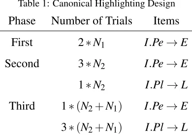
Table 1: Canonical Highlighting Design

Phase Number of Trials Items First 2∗N₁ I.Pe→E

Second 3∗N₂ I.Pe→E

1∗N₂ I.Pl→L

Third 1∗(N₂+N₁) I.Pe→E

3∗(N₂+N₁) I.Pl→L

Vandorpe, S., De Houwer, J., & Beckers, T. (2007). Outcome maximality and ad-ditivity training also influence cue competition in causal learning when learning involves many cues and events.Quarterly Journal of Experimental Psychology,

60, 356–368.

Vul, E., Goodman, N. D., Griffiths, T. L., & Tenenbaum, J. B. (2009). One and done? Optimal decisions from very few samples. InProceedings of the 31st Annual Conference of the Cognitive Science Society. Amsterdam, Netherlands.

8. Appendix

In this appendix we provide a description of the design of the canonical high-lighting experiment. The “canonical” design, shown in Table 1, equalizes the number ofI.Pe→E andI.Pl→Ltrials over the entire experiment. Within each phase the trials were randomly ordered. We used a canonical design in which

N1=10 andN2=5, repeating the experiment 100 times for each model to

Figure 2: Highlighting predictions for Globally Bayesian Learning (GBL), Locally Bayesian

Learning (LBL), and Factorized Bayesian Learning (FBL) for two experimental designs (explained

in the main text). Experimental results from Kruschke (2009) are plotted on each graph with

cir-cles. Error bars around the circles show 95% confidence intervals for the human data. The bar

plots show the model predictions of outcomeE, where the line marks equal preference between predictions ofE andL. A standard set of input cues is tested in each model: the original training sets of input cuesI.PeandI.Pl, as well as the critical tests of input cueI and input cuesPe.Pl. Each set of model predictions was made using the same parameters as used in Kruschke (2006b)

Figure 3: Blocking predictions for Globally Bayesian Learning (GBL), Locally Bayesian Learning

(LBL), and Factorized Bayesian Learning (FBL). Each bar plot shows the strength of theB→R

prediction after the control trials (C), after all of the forward blocking (FB) training trials, and after

all the backward blocking (BB) training trials. Each set of model predictions was made using the

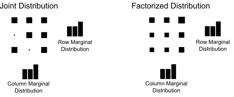
Figure 4: Example of a factorized distribution constructed from the marginals of a joint

distri-bution. Each cluster of nine boxes shows a joint probability distribution, where the probability

is equal to the area of a box (akin to a Hinton plot). The row of a box indexes the value of one

variable, while the column of the box indexes the value of a second variable. The bar plots are

Figure 5: Example comparison of the updating process of Globally Bayesian Learning (GBL)

and Factorized Bayesian Learning (FBL). Each cluster of nine boxes represents a joint probability

distribution, and probabilities are equal to the areas of the boxes (akin to a Hinton plot). The

column of a box indexes the setting of the first variable, while the row of the box indexes the

setting of the second variable. Within each gray area, GBL and FBL begin with the same prior

distributions and are updated with the same likelihoods. The left gray box shows the results of

updating GBL and FBL with a complex likelihood before a simple likelihood, while the right gray

box shows the results of updating GBL and FBL with the same likelihoods in the reverse order. At

the bottom of the figure, the final marginal distributions for each column are shown for FBL. The

difference plot at the bottom illustrates how sequential updating has produced order-dependent

Figure 6: Illustration of how the effects of highlighting arise from Factorized Bayesian Learning

(FBL). Each cluster of nine boxes shows a joint probability distribution, where the probability

is equal to the area of a box (akin to a Hinton plot). Each row within a cluster corresponds to

a different set of hypotheses about how the input cues activate the attended cues. Each column

within a cluster corresponds to how the attended cues activate the outcome. Each row of plots

corresponds to a different set of hypotheses. The first and second columns display the likelihoods

used in the first and second block of trials respectively. The third column displays the posterior

distributions of FBL following all training trials and the fourth column shows the final posterior

distributions again, but marginalized over the hypotheses about how input cues activate attended

Figure 7: Illustration of how the effects of blocking arise from Factorized Bayesian Learning

(FBL). Each cluster of nine boxes shows a joint probability distribution, where the probability

is equal to the area of a box (akin to a Hinton plot). Each row within a cluster corresponds to

a different set of hypotheses about how the input cues activate the attended cues. Each column

within a cluster corresponds to how the attended cues activate the outcome. Each row of plots

corresponds to a different training order condition. The first and second columns display the

likelihoods used in the first and second block of trials respectively. The third column displays the

posterior distributions of FBL following all training trials and the fourth column shows the final

posterior distributions again, but marginalized over the hypotheses about how input cues activate

Figure 8: Exclusive-OR (XOR) predictions for Globally Bayesian Learning (GBL), Locally

Bayesian Learning (LBL), and Factorized Bayesian Learning (FBL). Each bar plot shows the