http://wrap.warwick.ac.uk/
Original citation:
Borg, Matthew K., Lockerby, Duncan A. and Reese, Jason M.. (2013) Fluid simulations
with atomistic resolution : a hybrid multiscale method with field-wise coupling. Journal of
Computational Physics, Volume 255 . pp. 149-165. ISSN 0021-9991
Permanent WRAP url:
http://wrap.warwick.ac.uk/58527
Copyright and reuse:
The Warwick Research Archive Portal (WRAP) makes this work by researchers of the
University of Warwick available open access under the following conditions.
This article is made available under the Creative Commons Attribution 3.0 Unported (CC
BY 3.0) license and may be reused according to the conditions of the license. For more
details see:
http://creativecommons.org/licenses/by/3.0/
A note on versions:
The version presented in WRAP is the published version, or, version of record, and may
be cited as it appears here.
Contents lists available atScienceDirect
Journal of Computational Physics
www.elsevier.com/locate/jcp
Fluid simulations with atomistic resolution: a hybrid
multiscale method with field-wise coupling
✩
Matthew K. Borg
a,∗
, Duncan A. Lockerby
b, Jason M. Reese
aaDepartment of Mechanical & Aerospace Engineering, University of Strathclyde, Glasgow G1 1XJ, UK bSchool of Engineering, University of Warwick, Coventry CV4 7AL, UK
a r t i c l e
i n f o
a b s t r a c t
Article history: Received 12 April 2013
Received in revised form 7 August 2013 Accepted 10 August 2013
Available online 22 August 2013
Keywords:
Multiscale simulations Hybrid method Molecular dynamics Coupled solvers Scale separation
Newtonian and non-Newtonian flows Fluid dynamics
We present a new hybrid method for simulating dense fluid systems that exhibit multiscale behaviour, in particular, systems in which a Navier–Stokes model may not be valid in parts of the computational domain. We apply molecular dynamics as a local microscopic refinement for correcting the Navier–Stokes constitutive approximation in the bulk of the domain, as well as providing a direct measurement of velocity slip at bounding surfaces. Our hybrid approach differs from existing techniques, such as the heterogeneous multiscale method (HMM), in some fundamental respects. In our method, the individual molecular solvers, which provide information to the macro model, are not coupled with the continuum grid at nodes (i.e. point-wise coupling), instead coupling occurs over distributed heterogeneous fields (here referred to as field-wise coupling). This affords two major advantages. Whereas point-wise coupled HMM is limited to regions of flow that are highly scale-separated in all spatial directions (i.e. where the state of non-equilibrium in the fluid can be adequately described by a single strain tensor and temperature gradient vector), our field-wise coupled HMM has no such limitations and so can be applied to flows with arbitrarily-varying degrees of scale separation (e.g. flow from a large reservoir into a nano-channel). The second major advantage is that the position of molecular elements does not need to be collocated with nodes of the continuum grid, which means that the resolution of the microscopic correction can be adjusted independently of the resolution of the continuum model. This in turn means the computational cost and accuracy of the molecular correction can be independently controlled and optimised. The macroscopic constraints on the individual molecular solvers are artificial body-force distributions, used in conjunction with standard periodicity. We test our hybrid method on the Poiseuille flow problem for both Newtonian (Lennard-Jones) and non-Newtonian (FENE) fluids. The multiscale results are validated with expensive full-scale molecular dynamics simulations of the same case. Very close agreement is obtained for all cases, with as few as two micro elements required to accurately capture both the Newtonian and non-Newtonian flowfields. Our multiscale method converges very quickly (within 3–4 iterations) and is an order of magnitude more computationally efficient than the full-scale simulation.
©2013 The Authors. Published by Elsevier Inc. All rights reserved.
✩ This is an open-access article distributed under the terms of the Creative Commons Attribution License, which permits unrestricted use, distribution,
and reproduction in any medium, provided the original author and source are credited.
*
Corresponding author.E-mail addresses:[email protected](M.K. Borg),[email protected](D.A. Lockerby),[email protected](J.M. Reese). URL:http://www.micronanoflows.ac.uk(M.K. Borg).
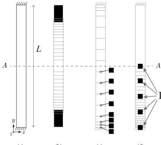
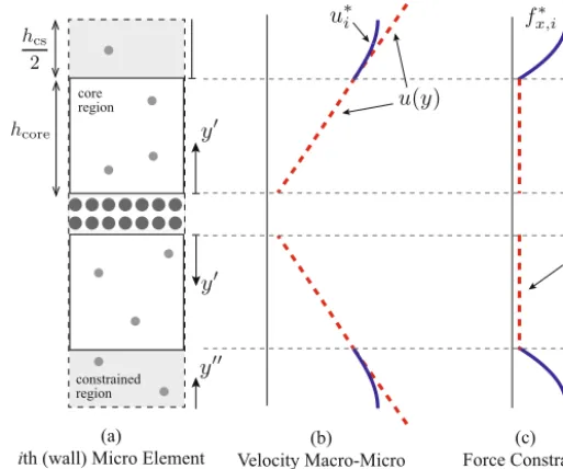
Fig. 1.Schematic of hybrid and multiscale methods in the literature, and our new multiscale approach proposed in this paper: (a) 1D Poiseuille flow problem; (b) Domain-Decomposition (DD); (c) Heterogeneous Multiscale Method (HMM) with point-wise collocated coupling; and (d) HMM with our Field-wise Non-collocated Coupling (HMM-FWC). The grey mesh indicates the macro domain, while black filled boxes indicate micro subdomains. A–Ais the line of symmetry.
1. Introduction
In an important class of fluid dynamics problems the overall physics is multiscale, in that microscopic processes strongly dictate the macroscopic behaviour. For example, granular flows in avalanches, shockwaves in high-speed rarefied flows, rain filtration through soil, etc. The present paper specifically focuses on micro- and nano-scale fluid dynamics, where atomistic processes occurring over pico- or nano-scales determine the bulk effects occurring over micro- and milli-scales, both temporally and spatially. The development of future technologies depending on nano- and micro-fluidics requires methods that resolve the multiscale phenomena accurately and efficiently.
Molecular Dynamics (MD) is now a recognised computational tool for accurately modelling fluid behaviour at atomistic scales as an ensemble of discrete molecules that obey fundamental laws of physics. In essence, a flow problem could be entirely described by such a microscopic model. While this is suitable for simulating small systems over short time-scales, such as water flows through carbon-nanotubes, in nano and micro engineering applications it becomes computationally intractable to resolve all the important space and time-scales involved.
In such flow problems, the continuum conservation laws can be used as an accurate, though incomplete, model for the macroscopic flow behaviour. Molecular dynamics can then be employed to replace, or close, equations in parts of the computational domain where a classical macroscopic constitutive or boundary model does not exist (e.g. liquids next to surfaces, rheological fluids, chemical reactions, etc). This is the so-called hybrid methodology, in which “the best of both worlds” in terms of computational cost and accuracy can be achieved by unifying disparate macroscopic and microscopic solvers in a coupled simulation.
The most common current approach to hybrid methods for dense fluids is domain-decomposition (DD) [1–6]. As the name implies, the computational domain is divided uniquely into macro and micro parts, providing only an overlapping region for matching hydrodynamic flux or state properties that act as Dirichlet or Neumann-type boundary conditions at the hybrid interface.Figs. 1(a) and (b) illustrate the DD method applied to a simple Poiseuille flow problem. Despite providing a reasonable rationale for modelling near-wall flows, DD schemes have some disadvantages. First, DD can only be used for flows that have a bulkflow region for which a constitutive model is known and is accurate. Furthermore, while it may be reasonably straightforward to segment a domain explicitly into micro/macro subdomains if it is a simple 1D system, it may be more challenging if the hybrid interface has more complex features[7]. Another issue is that of applying acceptable ‘open-system’ or ‘macro–micro’ boundary conditions at the non-periodic MD interface, which is a topic that is not well developed in the literature. Finally, DD methods do not generally work well for systems that exhibit varying degrees of scale separation, and can be of comparable computational cost to a full MD simulation of the case[8,9].
A different hybrid methodology that exploits the scale separation between molecular and continuum processes was proposed by E and co-workers[10,11]. This was dubbed the Heterogeneous Multiscale Method (HMM), and is illustrated in
information (such as shear-stress and slip) being provided by small independent MD elements distributed at the nodes of the computational mesh. These micro elements can be either bulk nodes or nodes on the boundary wall. Prior to supplying this information, every MD element is constrained using continuum fluid properties obtained at the nodal point, such as the strain tensor or the temperature gradient. Thispoint-wise coupling[12]between the computational grid and the individual molecular elements is valid for scale-separated conditions, where continuum property variations can be assumed to be small over the scale of the micro element (which has a small but finite size). In such conditions, the HMM approach naturally decouples processes occurring at different scales and can thus achieve major computational time savings over a full MD simulation.
The HMM has shown its potential in dense fluid simulations by various authors[12–14]. While these hybrid simulations all follow the original methodology proposed in[13](as described above), they differ from each other in the way the bulk-type micro elements are constrained from the local strain-rate (which is a second rank tensor) supplied by the continuum solution. For example, Ren and E [13]adopt a concept similar to the Lees and Edwards shear boundary condition [15]to impose a two-dimensional strain-rate. In principle each MD box is set to deform dynamically every MD time-step, based on the local macroscopic velocity field. A disadvantage of this deformation method is that the MD box may become too skewed, and the authors circumvent this by expensive MD reinitialisation steps. Yasuda and Yamamoto[14] instead apply a rotational transformation on the strain-rate tensor, to change it from the continuum co-ordinate system to a co-ordinate system more convenient for MD simulations. In particular, this transformation ensures that the diagonal terms of the new strain-rate tensor all become zero, which when applied to 2D isotropic problems gives only one non-zero strain-rate term in the off-diagonal. This means that the one-dimensional Lees and Edwards boundary method can then be conveniently applied without problems. The shear-stress tensor that is measured from the micro elements is then supplied back to the macro model after being transformed back to the original co-ordinate system. Asproulis et al.[12]strain the MD box using the Parrinello–Rahman deformation technique[16]in conjunction with the SLLOD algorithm[17]. This can be applied more generally to three-dimensional shearing because the local strain-rate is applied directly to the equations of motion of all molecules.
However, the second type of micro elements in HMM simulations provide the local wall boundary condition informa-tion, so the MD boxes are prohibited from adopting the same box-deformation methods as bulk micro elements. Instead, bounding boxes of wall micro elements are kept fixed, and velocity-type boundary conditions only are applied in a ‘con-trolling region’ next to the non-periodic boundary, in conjunction with periodic boundary conditions in the flow direction. In essence, there are therefore many similarities of HMM wall micro elements with DD schemes, such as that proposed by Hadjiconstantinou and Patera[2], i.e. a ‘Maxwell-Demon’ is applied only in the control region and it resamples new molecu-lar velocities from a Maxwell–Boltzmann distribution at the target continuum temperature and local velocity supplied from the overlaying continuum solution.
The biggest drawback of the HMM is that it is only suitable for completely scale-separated flow systems, due to the point-wise macro–micro coupling. For example, in simulations of water, a typical minimum MD element size is
xmicro
=
5 nm (to avoid wrap-around effects). For the HMM method to be worthwhile and not bemoreexpensive than full MD, the continuum grid spacing (xmacro) must then be at least greater than 5 nm, which represents a very severe restriction on the minimum scale of hydrodynamic variable variation that can be resolved with HMM in nano/micro-flows. Such a restriction precludes the use of HMM for technological applications that exhibit amixeddegree of scale separation, for example, where regions of the domain have characteristic scales much larger than the minimum MD scale (and where large savings can be made) and other regions have characteristic scales comparable to or smaller than the MD subdomains (e.g. a carbon nano tube connecting two reservoirs for filtration applications[18]).
Another significant drawback in HMM of the micro elements and macro nodes being collocated (i.e. there being a micro element at every continuum node) is that the micro and macro resolution are intrinsically linked. If the number of micro MD simulations are to be reduced, the macro resolution must be reduced, and vice versa. This may seem like a reasonable trade-off, given that generally in computational methods greater resolution comes with a computational penalty. However, in many cases this macro–micro link is unnecessarily restrictive and limiting. This is because, generally, micro MD elements provide the missing information to the macro model relating to stresses and heat-flux. But such quantities typically vary more slowly than the macro hydrodynamic variables of velocity, temperature and density, and thus will not necessarily require the same resolution. Consider the Navier–Stokes–Fourier constitutive relations: temperature and velocity variations are of a higher spatial-derivative order than the related heat flux and stress, respectively (e.g. in classical Poiseuille flow, the velocity profile is parabolic while the stress variation is linear). Although the Navier–Stokes–Fourier constitutive relations are not expected to hold fully at the nano scale, it is likely that the same tendency will exist. This means that, in general, lower resolution is required for the component of the simulation that is providing information to correct stress and heat flux (the micro elements) than is required of the component of the simulation resolving hydrodynamic variables (the macro grid).
scale separation (where hydrodynamic variables can vary substantially over the dimensions of a micro element) and allows the position of the micro elements to be optimised independently of the macro grid.
The remainder of this paper is structured as follows. In Section 2 we describe the new multiscale method in detail, providing a step-by-step account of the algorithm. In Section3we test the method on a simple and canonical flow problem for Newtonian and non-Newtonian fluids. In Section4we draw conclusions and discuss opportunities for further work.
2. A Heterogeneous Multiscale Method with Field-Wise Coupling (HMM-FWC)
As in conventional HMM, we adopt the fundamental notion that a continuum-fluid conservation model is applicable in the entire flow domain. However, instead of using MD to replaceconstitutive and boundary field data in the continuum model, we solve the macro description using a modified Navier–Stokes formulation; locally constrained micro simulations enter the hybrid formulation to provide constitutive and boundary-slipcorrectionsonly where needed.
For the current work we assume steady, incompressible and isothermal conditions, although the method is extensible to general flows. The governing three-dimensional macro-conservation equations for mass and momentum equations are:
∇ ·
U=
0,
(1)ρ
U· ∇
U+ ∇
p=
μ
∇
2U+
F+ ∇ ·
Ψ,
(2)whereU
=
(
u,
v,
w)
is the fluid velocity,ρ
is the mass density, pis the pressure,Fis a body force per unit volume,μ
is an assumed constant viscosity coefficient, andΨ
is a tensor field containing a correction to the Navier–Stokes constitutive model:Ψ
=
T−
2μ
e,
(3)where Tis the deviatoric stress tensor ande
=
12(
∇
U+ ∇
UT)
. The basic strategy of our multiscale method is to calculate an interpolated stress-correction fieldΨ
over the entire domain from evaluation of Eq. (3) at the distributed MD micro elements. From this,Uandpare then found from a solution to Eqs.(1)and(2).The primary characteristic of our method distinguishing it from HMM [13] is that coupling does not occur at every continuum node, but is applied over fields rather than points (compare Figs. 1(c) and (d)). As discussed in the previous section, the assumption underpinning point-wise coupling in HMM is not valid when the hydrodynamic variation occurs at the same spatial scale as the micro elements. In such cases, a direct physical correlation between macro and micro space is needed, requiring a flowfield of arbitrary complexity (e.g. a strain-rate field) to be simulated within each micro element. The imposition of this field on a micro element is not possible using techniques developed in the HMM literature, and so we propose a new constraint procedure that is consistent for both bulk and wall micro elements (explained in Sections2.3
and2.4below).
For the dual purpose of providing a detailed worked example, and also to prove the concept for a canonical flow, application of our method to an isothermal 1D Poiseuille flow geometry is described below. However, our underlying method is general, and may be extended to higher dimensions and other flow applications. We address the issues associated with advancing the method to two and three dimensions in the Conclusions section.
2.1. Overview of the algorithm
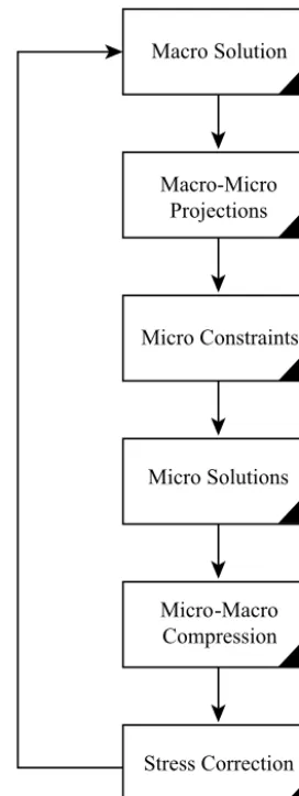
Our multiscale method is an iterative scheme that combines solutions from macro and micro solvers until a converged global solution is reached. The flow diagram of each sub-process in one multiscale iteration is illustrated in Fig. 2, and briefly described as follows:
1.Macro solution (see Section2.2) A solution to the continuum equations(1) and(2)is obtained for Uand p over the entire domain, with a stress-correction field
Ψ
taken from the previous iteration. Initially,Ψ
=
0.2.Macro-to-micro projections(see Section2.3) The macro solution isprojectedonto all micro subdomains. These projected flowfields serve as target conditions for the individual MD simulations to recreate. Each micro subdomain is divided into a ‘core’ region and a ‘constrained’ region. In the core region, the velocity field projection is a one-to-one mapping from the macro solution. In the constrained regions, however, the macro solution is modified so as to be compatible with the periodic boundary conditions of the MD elements; as such, it is only data obtained in the core regions that is physically accurate.
3.Micro constraints (see Section2.4) In order to generate the modified flow fields in the constrained regions of the MD subdomains (as obtained in Step 2), body-force distributions are used. The form and magnitude of the forces is cal-culated from the stress-corrected Navier–Stokes equations (1),(2), with the correction fields obtained in the previous iteration.
4.Micro solutions (see Section 2.5) Molecular dynamics simulations are started with the micro constraints (body-force distributions) calculated in Step 3 applied. Simulations are stopped after a predetermined period.1
1 Each micro element simulation at every iteration consists of two parts: the first part of the simulation allows the fluid to relax to the applied force
Fig. 2.Flow diagram of the iterative scheme.
5. Micro-to-macro compression(see Section2.6) Field measurements ofUandTare obtained from each micro element, and a least-squares polynomial fit is performed to extract continuous data.
6. Stress-correction(see Section2.7) The stress correction field
Ψ
is calculated from each micro element using Eq.(3)and interpolated over the entire macro domain, to be used in Step 1 of the next iteration. Other stress-correction fields are calculated for the constrained regions of the micro subdomains, for use in Step 3 of the next iteration.In the following sections we explain these six steps in detail, for the worked example of Poiseuille flow.
2.2. Macro solution (Step 1)
For the Poiseuille flow configuration ofFig. 1(a), the continuity equation (1)is automatically satisfied and the stress-correctedx-momentum equation(2)simplifies to:
0
=
μ
d2u
dy2
+
Fx+
d
Φ
dy
,
(4)where xis a coordinate in the streamwise direction, y is a coordinate across the channel, Fx is a body force driving the flow (which is constant for Poiseuille flow), and
Φ
(=
Ψ
xy) is a shear component of the stress-correction tensor:Φ
=
τ
xy−
μ
du
dy
,
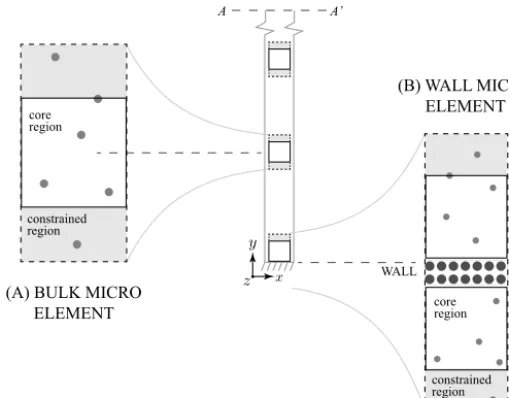
(5)Fig. 3.Domain partitioning of a Poiseuille flow problem into (A) bulk and (B) wall periodic micro elements. Grey and white regions indicate constraint and core regions respectively, while black dotted lines indicate periodic boundary conditions. A–Ais the line of symmetry; only one side of the channel is modelled by micro elements for this case.
where
τ
xy is the true shear-stress. Eq. (4) with Eq. (5) has no constitutive approximation and therefore holds for both molecular and continuum modelling treatments of the Poiseuille problem. In fact, the coupled equations are applicable even when the viscosity is not known exactly; an estimate forμ
will suffice, since the stress-correction termΦ
accommodates for any inaccuracies in the Navier–Stokes constitutive relation.A solution to Eq.(4)can be obtained for the Poiseuille flow case by integrating twice in the y-direction, over half the channel height H, giving a semi-analytical expression for the velocity profileu
(
y)
:u
(
y)
=
uB−
Fxy2
2
μ
+
y
μ
FxH+
1 2H
2H
0
Φ(
y)
dy−
1μ
y
0
Φ(
y)
dy.
(6)There are two unknowns in this expression: the stress correction field
Φ(
y)
, and the slip velocityuB. Initially both these are zero, but in subsequent iterations these properties are evaluated from the MD micro elements. We explain how these properties are measured and computed in Section2.6below. For more complex problems, where an analytical expression for fluid properties is not possible, the macro solution could be obtained using standard computational fluid dynamics (CFD), such as the finite volume method.Note, in the molecular simulations, the body force per unit volume Fx is converted to an actual force using: fx
=
Fx/
ρ
n, whereρ
nis the number density.2.3. Macro–micro projection (Step 2)
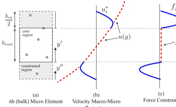
The aim of the field-wise coupling approach is for the individual micro elements (see Fig. 3) to reproduce the same flowfield that occurs over the corresponding region in the continuum domain. To this end, the estimated macroscopic velocity fieldu
(
y)
, which is obtained from the stress-corrected momentum Eq.(4), is projected onto the domain of each micro element. This projection is indicated by the red dashed line in Fig. 4(b). This projection is then modified in the ‘constrained’ regions, in order to be consistent with the periodic boundary conditions2 of the MD solver (see solid blue line in Fig. 4b). In these constrained regions, where the velocity profile has been artificially modified, body forces are applied (calculated in the next step, Section 2.4) in order to reproduce the modified velocity profile. No artificial body-forcing is applied in the core regions.The flow velocity projection (denoted by the superscript∗) in the core region of theith micro element (u∗i) is obtained directly from the macro solution, i.e.
u∗i
=
uyi for 0<
yi<
hcore, (7)where yi is a new local co-ordinate system used to identify the core region, as indicated inFig. 4. The height of the core region is denoted byhcore.
Fig. 4.Illustration of (a) abulkmicro element, (b) the projection of the macro velocity solution in the constrained regionu∗i and (c) the consistent force
constraint in the constrained region fx∗,iderived from the velocity projection. In figures (b) and (c) solid lines indicate periodic-projections, while dotted lines indicate unmodified macro fields.
In the constrained region the velocity projection is modified with the intention of bridging the velocities at the two sides of the core region with a continuous velocity field (as well as continuous first and second derivative velocity fields) that pass through the top and bottom periodic boundaries.
To preserve continuity over the two interfaces of velocity and its first and second derivative, a sixth order polynomial is used:
u∗i
yi=
6
k=1
ak,iyi(M−k) for 0
<
yi<
hcs, (8)where yi is a different local co-ordinate system used to identify the constrained region (see Fig. 4), hcs is the height of the constrained region, and ak,i are the polynomial coefficients which are uniquely determined through the following six boundary conditions:
u∗i
=
u,
du ∗ idyi
=
du dy,
andd2u∗ i
dyi2
=
d2udy2
,
at bothyi=
0 andyi=
hcs. (9)For the micro elements touching the walls of the Poiseuille flow problem, there are issues of non-periodicity. All that is then required to be able to use periodic boundary conditions is for the wall micro element to be a symmetrical flow domain with the line of symmetry running through the constrained region or wall, as shown inFig. 5(a). The velocity projection for the wall micro element, both for the core and constrained regions, are identical to those in the bulk micro elements and can be similarly calculated using Eqs.(7)and(8), as illustrated inFig. 5(b).
2.4. Micro constraints (Step 3)
The modified flowfield of the constrained regions can be generated using an artificial body force fx∗, as shown inFigs. 4(c) and 5(c) for bulk and wall micro elements respectively. To calculate this force distribution we substitute the target velocity field(8)into the flux-corrected Navier–Stokes Eq.(4):
fx∗,i
= −
1ρ
nd
Φcs
,idy
−
μ
ρ
nd2u∗i
dy2
,
for 0<
yi<
hcs, (10)where
Φ
cs,i is the stress correction field in the constrained region of theith subdomain and is calculated in the previous iteration (Step 6, Section2.7). Note, in the initial iterationΦ
cs=
0.In the core regions of the micro subdomains, molecular dynamics is performed without any additional artificial forcing imposed. As such, the forcing in the core region takes that of the Poiseuille driving force only, i.e.
fx
=
Fx
ρ
nFig. 5.Illustration of (a) awallmicro element, (b) the projection of the macro velocity solution in the constrained regionu∗i and (c) the consistent force
constraint in the constrained regionfx∗,i derived from the velocity projection. In figures (b) and (c), solid lines indicate periodic-projections, while dotted lines indicate unmodified macro fields.
2.5. Micro solution (Step 4)
All our micro elements are simulated using the open source non-equilibrium Molecular Dynamics code,mdFoam[7,19, 20], which is implemented within OpenFOAM’s C++ libraries[21]. Detached micro elements located in the bulk of the flow domain (bulk elements, see Fig. 3) each consist of a fully-periodic domain that is filled solely with fluid molecules at the target density and temperature defined by the problem. The micro element next to the channel bounding surface (wall elements, seeFig. 3) also include wall–material molecules, which are modelled as rigid atoms with parameters chosen from
[22]to generate a reasonable slip behaviour.
For the duration of the simulation, all fluid molecules in each micro element evolve according to Newton’s equations of motion:
d
dtrk
=
vk,
(12)mk
d dtvk
=
f
k
+
fextk,
(13)wherek
=
(
1, . . . ,
N)
is a particular molecule in the system ofN molecules,mkis the molecule mass,rk=
(
xk,
yk,
zk)
is its position, andvk=
(
uk,
vk,
wk)
is its velocity. The total intermolecular forcefkin Eq.(13)is computed from pair forces with neighbouring molecules by:fk
=
N
j=1(=k)
−∇
U(
rkj),
(14)where U
(
rkj)
is the interaction potential between fluid–fluid or solid–fluid interactions. For simplicity we simulate monatomic liquid argon using the 12-6 Lennard-Jones (LJ) potential (although water or other molecules can also be simu-lated straightforwardly, as we demonstrate in Section3.2for a polymeric fluid):UL J
(
rkj)
=
4σ
rkj
12−
σ
rkj
6,
(15)where
=
1.
6568×
10−21J andσ
=
0.
34 nm are the potential’s characteristic energy and length scales, andrkj= |
rk−
rj|
is the separation of two arbitrary molecules (j,
k) within a cut-off radius, rcut=
1.
36 nm. The equations of motion are numerically discretised in space and time using a time-steptthat is 5.4 fs for the LJ simulations in Section3.1, and 2.2 fs for the FENE chain simulations in Section3.2.
The termfextk in Eq.(13)is alocally-applied external force derived from the constraint step (Step 3, Section2.4). In this fluid problem,fext
(
y)
=
fx∗,i(
y)
nˆ
xis a force distribution applied in the constrained region according to the macro–micro con-straint(10), andfext=
fin the streamwise x-direction. In order to maintain isothermal conditions, the heat introduced by the induced shearing is removed using a velocity unbiased Berendsen thermostat[23]in bins of 0.68 nm thickness in the y-direction.
The size of the constrained region is picked for convenience to be the same as that of the core region. This produces strain-rates in both regions that are of similar magnitude, and thus places similar requirements on the thermostat. Almost certainly this region could be shrunk for greater computational savings with no penalty in accuracy. However, if the region is chosen to be excessively small (e.g.
∼
1 molecular diameter), an extremely large rate of strain is applied locally, which in turn will generate an amount of heat that would be extremely difficult to remove homogeneously using the thermostat.2.6. Micro compression (Step 5)
After all micro elements reach a relaxed steady-state, measurements are obtained using a cumulative averaging technique to reduce noise. Each micro element is divided into spatially-oriented bins in the y-direction in order to resolve the velocity and shear-stress profiles. Velocity in each bin is measured using the Cumulative Averaging Method (CAM) [24], while the stress tensor field is measured using the Irving–Kirkwood relationship [25]. A least-squares polynomial fit to the data is performed, which helps reduce noise further. The fit produces a continuous function that avoids stability issues arising from supplying highly fluctuating data to the macro solver. A least-squares fit is applied to an Nth order polynomial for the velocity profile in the core region, and anMth order polynomial for the velocity profile in the constrained region:
ui,core=
Nk=1
bk,iyi(N−k)
,
for 0yihcore, (16)and
ui,cs=
Mk=1
ck,iyi(M−k)
,
for 0yi hcs, (17)wherebk,iandck,iare the coefficients of the polynomials used in the core micro region and constrained region respectively. An estimate of the new slip velocity uB for input to the macro solution (6)is taken directly from the compressed wall micro-element solution(16), atyi
=
0.Shear-stress least-squares fits in the core and constrained regions are similar to Eqs.(16)and(17), but with one polyno-mial degree less, i.e.
τ
i,core=
N−1k=1
dk,iyi(N−1−k)
,
for 0yihcore,
(18)and
τ
i,cs=
M−1
k=1
ek,iyi(M−1−k)
,
for 0yi hcs. (19)Values forN andM are taken to be 3 and 6, respectively, for all our hybrid simulations.
2.7. Stress correction (Step 6)
The stress correction fields in both the core
Φ
i,core(
y)
and the constrainedΦ
i,cs(
y)
regions can be calculated using Eq.(5)for each micro domain, i.e.Φ
i=
τ
xy−
μ
d
udy
,
(20)where angle bracket terms on the right hand side are obtained from Eqs.(16)–(19).
The final step is to interpolate the flux correction field from the core region of all micro elements onto the entire macro domain, i.e. over what we refer to as the ‘macro gaps’, as shown inFig. 6. To do this we use a Qth-order polynomial:
Φ
i,gapy
=
Q
k=1
gk,iyi (Q−k)
,
for 0yi hi,gap,
(21)Fig. 6.Illustration of macro gaps (dark regions) over which the stress correction is interpolated.
2.8. Iteration and convergence
Updated continuum solutions u
(
y)
are obtained at each iteration of the algorithm, until convergenceul−1→
ul, wherel is the iteration index. Here we use a simple convergence expression based on solutions ofuof the following form:ζ
=
1NP NP
j
u(
yj)
l−
u(
yj)
l−1u
(
yj)
lζtol,
(22)whereNP are the number of macro nodes and
ζ
tolis a pre-specified tolerance parameter.3. Results
3.1. Validation test for a Newtonian fluid
The HMM-FWC algorithm is now tested on the Poiseuille flow of a Lennard-Jones fluid, such that the choice of state point and maximum strain-rate gives a Newtonian response. The capability of our method is shown by intentionally choosing the viscosity that is input to the macro solution to be
∼
40% smaller than the actual viscosity at the target density and temperature of the problem. We show how our method corrects for this mismatch of viscosity (i.e. the micro solution corrects the macro solution) indirectly through the stress-correction field.The Poiseuille channel height, L
=
162 nm, is chosen small enough in this test case so that results from our hybrid simulation can be compared and validated against a full MD simulation (which is very computationally expensive). Com-putational savings of the hybrid method over full MD will be far greater for larger and more realistic nano and micro flow problems.The description of the fluid (state, potentials, thermostat) and bounding wall (packing, lattice-structure, potential) need to be the same for both full MD and hybrid simulations for a fair comparison of accuracy to be made. The potential properties for the liquid–liquid and wall–liquid interactions are taken from Ref. [22], with the intention to generate slip at the solid–liquid interface. The values for these are,
σ
l−l=
3.
4×
10−10m,l−l
=
1.
65678×
10−21J andσ
w−l=
2.
55×
10−10m,w−l
=
0.
33×
10−21J in Eq. (15). The solid wall is chosen to be a simple cubic lattice-structure, with number density 5.
5×
ρ
n, whereρ
n=
1437 m−3 is the fluid number density. The mass of liquid atoms isml=
6.
6904×
10−26kg. In the full MD description, there are 103,593 liquid molecules and 9464 wall molecules. The macro force fx=
4.
872 fN and Berendsen thermostat at T=
292.
8 K are applied to the equations of motion of all molecules until a steady-state solution is reached (after∼
300 ns of problem time). The steady-state full velocity profile is then averaged over 2 ns.Fig. 7.Overview of the Poiseuille flow channel case using three different hybrid simulations (a, b, c) with varying number of micro elements (Π=1,2,3) and locations. Insets on the right are the bulk and wall micro element MD simulations — dashed lines indicate periodicity, and lightened regions indicate the constrained regions.
Fig. 8.Predictions of the half-channel velocity profile for three hybrid Poiseuille flow simulations: (a)Π=1, (b)Π=2, and (c)Π=3, at iteration l=3. The multiscale results () are compared to the steady full MD simulation (—) and the Navier–Stokes solution with zero slip and initial viscosityμest
(N.S.*,).
interpolant polynomial in Eq.(21)because the flow is Newtonian in the whole computational domain, so we expect a linear stress-correction. A higher polynomial order can also be used, but this increases noise-related oscillations in the overall result. A tolerance value of
ζ
tol=
0.
01 was chosen for this test case to determine convergence, and this was obtained in all three hybrid simulations after only 3 iterations.The converged results for velocity profiles from the hybrid simulations are presented in Fig. 8. Velocity profiles from all three hybrid cases match very well with the steady-state velocity profile measured from the full MD simulation. Also plotted in the figures are the velocity profiles predicted by the no-slip Navier–Stokes solution (with the initial estimated viscosity
μest
). We confirm from these results that the 40% lower viscosity that is chosen as an initial guess does not affect the final hybrid solution. [image:12.561.92.451.330.481.2]Fig. 9.Hybrid predictions of the half-channel stress-correction fieldΦ(y)forΠ=1 (),Π=2 (), andΠ=3 () at iterationl=3. Comparison are made with calculations taken from the full MD simulation (—) using Eq.(20).
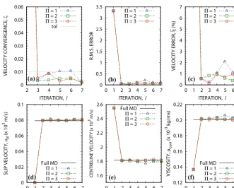
Fig. 10.Accuracy and convergence results for hybrid simulations withΠ=1 (),Π=2 (), andΠ=3 () micro elements, against iteration numberl. Comparisons are made with the full MD simulation (—). (a) Convergence of velocity, computed using Eq.(22). (b) R.M.S. error, computed using Eq.(23). (c) Local mean velocity error between hybrid and full MD profiles, computed usingξ=1/NpNpξ(y), whereξ(y)= [uF(y)−uH(y)]/uF(y)×100%.
(d) Slip velocity. (e) Centreline velocity. (f) Corrected bulk viscosityμcorr, calculated from Eq.(25).
example remains Newtonian. Fluctuations in the calculation of
Φ
in the hybrid simulations stem from the noise inherent in the micro MD simulations.InFig. 10we present an overview of the most important accuracy and convergence results of our hybrid simulations. No major instabilities in the hybrid algorithm were observed when simulations were run beyond the converged iterationl
=
3.Fig. 10(a) shows the convergence parameter
ζ
, which is calculated from the velocity profiles at two successive iterations using Eq. (22); after the third iteration, all three cases lie below the pre-specified tolerance valueζ
tol=
0.
01. InFig. 10(b) we present a measure of accuracy for the overall velocity profile for all three hybrid simulations when compared to the full-scale simulation, using a root-mean-square (R.M.S.) estimate at each iteration step:R.M.S. error
=
1Np Np
j
uF
(
j)
−
uH(
j)
2 [image:13.561.110.442.239.505.2]where uF, uH are the full MD and hybrid velocity solutions respectively, and Np are the number of macro nodes. The predicted R.M.S. errors are very close to zero for all cases. Similarly in Fig. 10(c) we present the percentage errors and show that these are less than 1% for
Π
=
2,
3 and less than 2% forΠ
=
1. There are only marginal differences between the three hybrid cases, and so we can be confident that the solution of the Poiseuille flow of a Newtonian fluid could be obtained using just one wall micro element (Π
=
1), with additional elements not improving the accuracy of the prediction substantially. Note that in conventional HMM (using point-wise coupling) the minimum number of subdomains is equal to the number of grid points in the macro domain (here, it would be over 4000).The slip velocity uB in Eq. (6) and the velocity in the midpoint of the channel are presented in Figs. 10(d) and (e) respectively. Again, there is excellent agreement between the full-scale MD simulation and the hybrid results for all three cases.
To verify that we get an accurate prediction of viscosity from the hybrid simulation, we assume that the stress correction has the same form as the Navier–Stokes relationship, i.e.,
Φ
= ˜
μ
dudy
,
(24)where
μ
˜
is the missing contribution of viscosity. Eq.(24)can be numerically integrated to calculate a corrected viscosity:μ
corr= ˜
μ
+
μ
est, (25)which is then plotted against the viscosity measured in the full MD simulation inFig. 10(f). Again, there is good agreement in the viscosity prediction
μcorr
between our hybrid approach and the full MD solution.3.2. Validation test for a non-Newtonian fluid
There are many applications in the polymer processing industry where accurate predictions of flows of various rheologically-complex fluids, such as polymer solutions and polymer melts, are important[12,26]. One of the main chal-lenges associated with modelling these fluids is that even if the non-linear relationship between shear-stress and strain-rate is known, we are still left with a system of partial differential equations that is often too complex to solve numerically[26]. An alternative to continuum fluid modelling is therefore to adopt a model of the fluid’s molecular constituents, and solve the flow using non-equilibrium MD simulations[26,27].
In this section we demonstrate the capability of our multiscale method for a polymer fluid. The method is properly tested by choosing operational strains in a regime where the relationship with shear-stress is highly non-linear, thus imposing a non-linear variation of viscosity throughout the entire computational domain.
The test fluid in this case consists of a pseudoplastic polymer that is modelled artificially in MD using dumb-bell chains of NB connected ‘beads’ (that replace the notion of atoms) [26]. Every bead in the chain is connected to another via a finitely extensible non-linear elastic (FENE) potential, which is expressed as:
UFENE(rkj
)
=
−
0.
5kr02ln[
1−
(
rkjr0
)
2
]
ifr kj<
r0,
∞
ifrkjr0,(26)
wherek
=
0.
43 kg s−2 is the FENE spring constant andr0=
5.
1 Å is the finite extensibility of a pair of connected beads. These properties are chosen from Refs.[12,28]in order to minimise bond cross-overs. Here we choose a fluid withNB=
10 beads per chain, at a bead density ofρ
n=
1447 m−3 and temperatureT=
292.
8 K. A Lennard-Jones potential(15)is also applied in a similar way as before between all neighbouring beads within the cut-off distance.The same Poiseuille flow case as in Section3.1 is used here to test our multiscale method for non-Newtonian flows. Properties of the setup remain the same as before, except when explicitly stated. The dimensions
x
=
z
=
6.
8 nm are made larger for both the full MD and hybrid cases in order to allow enough distance for one chain not to interact with itself across the periodic boundaries if fully extended (∼
4.6 nm). As a result, the number of molecules in the full MD was increased to 166,274 (with 2592 wall molecules), 22,666 molecules in the wall micro element, and 13,526 molecules in every bulk micro element. The macro force was also increased to fx=
24.
36 fN in order to operate the fluid in a non-linear stress-strain regime, as discussed above. To control the level of slip at the wall we have reduced the wall density to that of the fluid, and modified the wall–liquid LJ parameters toσ
w−l=
3.
4×
10−10m,w−l
=
0.
995×
10−21J, as suggested in[22]. The full MD case is set up by first initialising the channel height with the target number of beads corresponding to the target density, followed by a short simulation until all chains are grown to the correct bead-length. The gravity-type forcing, i.e. fx=
24.
36 fN is then applied until a steady-state is reached (after∼
130 ns of problem time), followed by a short simulation period for measurement (lasting∼
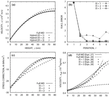
1 ns).Fig. 11.Results for the non-Newtonian multiscale simulations forΠ=1 (),Π=2 (), andΠ=3 () micro elements: (a) cross-channel velocity profile; (b) R.M.S. errors vs iteration; (c) stress correction field; (d) effective viscosity field.
All our hybrid simulations converge in 3–4 iterations, to a tolerance of
ζ
tol=
0.
02. The channel velocity profiles are presented in Fig. 11(a), while the overall error plots are displayed in Fig. 11(b). Excellent agreement is found between the full-scale MD simulation and the hybrid simulations forΠ
=
2 andΠ
=
3 micro elements (less than 1% difference). However, less good agreement is found for the hybrid case with just one wall micro element (Π
=
1), which oscillates between 2–7% of the full MD result; inaccuracies are caused by the lack of micro resolution in the bulk, whereas near-wall predictions (such as slip and stress) match just as well as in the higherΠ
cases. This can also be observed in the overall stress-correction fieldΦ
in Fig. 11(c), which, unlike before, now varies non-linearly. Note that there is no actual stress correction in the full MD simulation, but as before we estimate it using the equivalent of Eq. (20)with the shear-stressτ
xyF and velocityuF profiles measured from the full MD simulation.To evaluate an ‘effective viscosity’ field
μeff
for both hybrid and full-scale simulations, we use the Oswald–de Waele relationship:τ
xy=
μ
eff∂
u∂
y.
(27)The full MD viscosity field is evaluated directly from this expression using the stress
τ
xyF and velocityuF measurements. For the hybrid simulation, Eq.(27)must first be substituted in the corrected Navier–Stokes Eq.(5)to give:μ
eff(y)
=
μ
est+
Φ
∂
u∂
y −1.
(28)Calculations of effective viscosity are plotted in Fig. 11(d). Again, there is good agreement between the full-scale MD and the hybrid calculations adopting
Π
=
2,
3 micro elements, but poor agreement for theΠ
=
1 case in the bulk of the channel. Good agreement is also obtained with the standard power-law relationship:μ
eff≈
K∂
u∂
y −a,
(29)wherea is the flow behaviour index (a
<
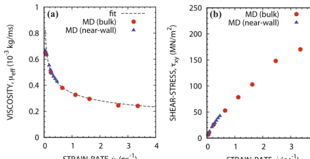
1 for pseudoplastic fluids) and K is the flow consistency index. The values foraFig. 12.Pure MD results for a FENE fluid under various strain-rates (γ˙=du/dy) next to a bounding wall () and in bulk-fluid elements (•): (a) effective viscosity against strain, and (b) stress against strain. Also plotted in (a) is a power-law fit through the data points using Eq.(29).
state, under various strain-rates. Effective viscosity vs strain-rate and shear-stress vs strain-rate are plotted inFigs. 12(a) and (b), respectively. In these simulations we obtained fit values fora
=
0.
275 andK=
5.
3×
10−7Pa sa.3.3. Computational savings
We now present the computational savings that our HMM-FWC method has afforded over the full-scale MD simulations by computing the total processing time P
=
total number of time-steps×
average processing time per time-step, for both approaches. For the full MD simulation this is simply:PF
=
tc,F(
ttran,F+
tav,F)/
t,
(30)wheretc,F is the average clock time per MD time-step,ttran,F is the transient time required for the flow to develop from rest to steady-state,tav,F is the averaging-time required to reduce noise from molecular measurements and
t is the MD time-step. For the hybrid method the total processing time is:
PH
=
Itc,W
(
ttran,W+
tav,W)
+
tc,B(
ttran,B+
tav,B)(Π
−
1)
/
t,
(31)where subscripts W and B refer to the wall and bulk micro elements respectively, and I is the number of iterations at which the hybrid algorithm converges (I
=
3 in Section 3.1 and I=
4 in Section 3.2). The cumulative averaging times are the same for all MD cases, sotav,F=
tav,W=
tav,B=
tav (tav≈
9 ns in Section3.1, whiletav≈
2 ns in Section3.2). The transient times are, however, dependent on the size of the MD domains. For example, in the Newtonian case Section3.1, the transient time in the hybrid simulation isttran,W=
ttran,B=
2 ns, while the full MD suffers from a very long start-up timettran,F
≈
300 ns.3 Not having to simulate this long transient period is a major computational advantage of our multiscale approach for studying steady-state flows. In the non-Newtonian casettran,W=
ttran,B=
1 ns, whilettran,F≈
130 ns.The ratio of Eqs.(30)to(31)gives the total computational speed-up factor,c
=
PF/
PH. For the cases in Section3.1, the average clock times measured for the wall and bulk micro elements were:tc,W=
0.
0326 s andtc,B=
0.
015 s respectively, while the full MD simulation measured a clock time oftc,F=
0.
251 s. So this means 74×
, 50×
and 38×
speed-ups for the hybrid cases withΠ
=
1, 2 and 3 micro elements respectively. For the cases in Section3.2, the average clock times were:tc,W
=
0.
059 s,tc,B=
0.
033 s andtc,F=
0.
595 s, which means 100×
, 66×
and 49×
speed-ups for the non-Newtonian cases withΠ
=
1, 2 and 3 micro elements, respectively. Clearly our hybrid method is very computationally efficient.4. Conclusions
We have proposed a new multiscale method that differs from the previous Heterogeneous Multiscale Method (HMM)
[13]by employing a field-wise macro/micro coupling (as opposed to a point-wise coupling at every macroscopic node). This enables a greater range of scales over which our method can be applied, which is essential for the modelling of practical nano and micro flow systems. The ability to decouple the positions of the micro elements from the macro grid nodes affords major computational savings (in both examples presented here, excellent results were obtained with as few as two micro elements). The field-wise coupling method is implemented using a novel macro/micro constraint procedure that involves
3 This start-up time can be reduced by initialising the system with a velocity profile as close as possible to the final solution, if this is known (for
calculating stress-corrections to the standard Navier–Stokes equations, and projections of flowfields of arbitrary complexity on bulk- and wall-type micro elements.
We have simulated both Newtonian and non-Newtonian Poiseuille flows, and the multiscale method gives flow predic-tions in close agreement with full-scale MD simulapredic-tions of the same cases. The method converged very quickly, within 3–4 iterations, which is an attractive feature for extending it to study quasi-steady transient problems, as described in Ref.[29]. While the Newtonian flow case showed that having just one wall micro element is sufficient to produce accuracies within 1–2% of the full result, we found that in the non-Newtonian case at least one bulk micro element and one wall micro element were required to capture the significant variation of viscosity produced by a FENE fluid under high strain-rates. Our multiscale method is approximately 74
×
and 66×
more computationally efficient than full MD simulations of the Newtonian and non-Newtonian cases, respectively.The HMM-FWC method presented in this paper can be extended to two- and three-dimensional flow problems. How-ever, the method becomes more complicated and there are some particular issues that need to be addressed carefully. In 3D flows, for example, MD micro elements are constructed with a constraining region that surrounds the core region completely (instead of the top–bottom approach for 1D flows), and the micro constraint forces are a 3D varying field. The accurate application of this force field is paramount, so a fine 3D mesh is required, which is costly. Similar issues arise for the macro-to-micro projection step and the micro compression step — high order interpolants are required to provide veloc-ity projections and fits through measurements of shear-stress and velocveloc-ity taken from the MD core region. In the projection step there is also the issue of preserving continuity in the core-constrained region (which is not necessarily straightfor-ward). Furthermore, in the micro MD simulations there is an exacerbated problem of noise, as smaller bins are required to capture 3D gradients, which may lead to instabilities in the hybrid algorithm if the measured fields are not sufficiently averaged. For the one-dimensional examples considered in the present paper, mass is automatically conserved, leaving only the momentum conservation Eq.(2)to be solved macroscopically. For more general flow problems, a macroscopic continuity equation must also be solved alongside an equation of state relating density to pressure. The induced pressure variations would then be coupled to the momentum conservation equation using a distributed force field. The development of the HMM-FWC method to higher-dimensional flow problems is therefore the subject of future work.
Acknowledgements
This work is financially supported in the UK by EPSRC Programme Grant EP/I011927/1. Our calculations were performed on the high performance computer ARCHIE at the University of Strathclyde, funded by EPSRC grants EP/K000586/1 and EP/K000195/1.
References
[1]S.T. O’Connell, P.A. Thompson, Molecular dynamics-continuum hybrid computations: A tool for studying complex fluid flows, Phys. Rev. E 52 (1995) R5792–R5795.
[2]N. Hadjiconstantinou, A. Patera, Heterogeneous atomistic-continuum methods for dense fluid systems, Int. J. Mod. Phys. C 8 (1997) 967–976. [3]G. Wagner, E. Flekkøy, J. Feder, T. Jøssang, Coupling molecular dynamics and continuum dynamics, Comput. Phys. Commun. 147 (2002) 670–673. [4]R. Delgado-Buscalioni, P.V. Coveney, Continuum-particle hybrid coupling for mass, momentum, and energy transfers in unsteady fluid flow, Phys. Rev.
E 67 (2003) 1–13.
[5]X.B. Nie, S.Y. Chen, W. E, M.O. Robbins, A continuum and molecular dynamics hybrid method for micro- and nano-fluid flow, J. Fluid Mech. 500 (2004) 55–64.
[6]T. Werder, J.H. Walther, P. Koumoutsakos, Hybrid atomistic-continuum method for the simulation of dense fluid flows, J. Comput. Phys. 205 (2005) 373–390.
[7]M.K. Borg, G.B. Macpherson, J.M. Reese, Controllers for imposing continuum-to-molecular boundary conditions in arbitrary fluid flow geometries, Mol. Simul. 36 (2010) 745–757.
[8]M.K. Borg, D.A. Lockerby, J.M. Reese, A multiscale method for micro/nano flows of high aspect ratio, J. Comput. Phys. 233 (2013) 400–413.
[9] M.K. Borg, D.A. Lockerby, J.M. Reese, A hybrid molecular-continuum simulation method for incompressible flows in micro/nanofluidic networks, Mi-crofluid. Nanofluid. (2013),http://dx.doi.org/10.1007/s10404-013-1168-y.
[10]W. E, E. Bjorn, H. Zhongyi, Heterogeneous multiscale method: A general methodology for multiscale modeling, Phys. Rev. B 67 (2003) 092101. [11]W. E, B. Engquist, The heterogeneous multiscale methods, Commun. Math. Sci. 1 (2003) 87–132.
[12]N. Asproulis, M. Kalweit, D. Drikakis, A hybrid molecular continuum method using point wise coupling, Adv. Eng. Softw. 46 (2012) 85–92. [13]W. Ren, W. E, Heterogeneous multiscale method for the modeling of complex fluids and micro-fluidics, J. Comput. Phys. 204 (2005) 1–26. [14]S. Yasuda, R. Yamamoto, A model for hybrid simulations of molecular dynamics and computational fluid dynamics, Phys. Fluids 20 (2008) 113101. [15]A.W. Lees, S.F. Edwards, The computer study of transport processes under extreme conditions, J. Phys. C, Solid State Phys. 5 (1972) 1921–1928. [16]M. Parrinello, A. Rahman, Polymorphic transitions in single crystals: A new molecular dynamics method, J. Appl. Phys. 52 (1981) 7182–7190. [17]D.J. Evans, G.P. Morriss, Statistical Mechanics of Nonequilibrium Liquids, Academic Press, 1990.
[18]W.D. Nicholls, M.K. Borg, D.A. Lockerby, J.M. Reese, Water transport through (7, 7) carbon nanotubes of different lengths using molecular dynamics, Microfluid. Nanofluid. 12 (2012) 257–264.
[19]G.B. Macpherson, M.K. Borg, J.M. Reese, Generation of initial molecular dynamics configurations in arbitrary geometries and in parallel, Mol. Simul. 33 (2007) 1199–1212.
[20]G.B. Macpherson, J.M. Reese, Molecular dynamics in arbitrary geometries: Parallel evaluation of pair forces, Mol. Simul. 34 (2008) 97–115. [21] OpenFOAM,www.openfoam.org, 2013.
[22]P.A. Thompson, S.M. Troian, A general boundary condition for liquid flow at solid surfaces, Nature 389 (1997) 360–362.
[23]H.J.C. Berendsen, J.P.M. Postma, W.F. van Gunsteren, A. Dinola, J.R. Haak, Molecular dynamics with coupling to an external bath, J. Chem. Phys. 81 (1984) 3684–3690.
[25]J.H. Irving, J.G. Kirkwood, The statistical mechanical theory of transport processes. IV. The equations of hydrodynamics, J. Chem. Phys. 18 (1950) 817–829.
[26]B.Z. Dlugogorski, M. Grmela, P.J. Carreau, Viscometric functions for Fene and generalized Lennard-Jones dumbbell liquids in Couette flow: molecular dynamics study, J. Non-Newton. Fluid Mech. 48 (1993) 303–335.
[27]J.W. Rudisill, P.T. Cummings, The contribution of internal degrees of freedom to the non-Newtonian rheology of model polymer fluids, Rheol. Acta 30 (1991) 33–43.
[28]M. Kröger, S. Hess, Rheological evidence for a dynamical crossover in polymer melts via nonequilibrium molecular dynamics, Phys. Rev. Lett. 85 (2000) 1128–1131.