Approximate Least Squares Accelerator
MSc Thesis
Alexander Krapukhin
Committee:
Dr.ir. A.B.J. Kokkeler
S.G.A. Gillani
Ir. J. Scholten
Computer Architecture for Embedded Systems Faculty of Electrical Engineering, Mathematics and Computer Science University of Twente Enschede The Netherlands
2
Contents
Abstract. ... 4
Introduction.... 5
1. Literature review. ... 7
1.1. Error resilience analysis. ... 7
1.2. Approximate computing techniques. ... 12
2. Multiply-accumulate unit and its approximation. ... 15
2.1. Least Squares Problem ... 15
2.2. Multiplier-accumulator (MAC) ... 16
2.3. Unit gate model ... 18
2.4. Errors and error metrics. ... 19
2.5. Mitigation of errors. ... 23
2.5.1. Mean error balancing. ... 23
2.5.2. Using two multipliers with opposite errors. ... 23
2.5.3. Accumulator initialization. ... 24
2.6. Approximate units against careful data sizing. ... 25
2.7. Approximate multipliers for MAC. ... 26
2.7.1. Recursive approximate multipliers ... 26
2.7.2. Dynamic Range Unbiased Multiplier (DRUM). ... 34
2.7.3. Low-Power Approximate MAC Unit. ... 36
2.7.4. Approximate Booth multiplier. ... 37
3. Comparison of approximation methods. ... 39
3.1. Experimental setup for comparisons. ... 39
3.2. Comparison results. ... 44
3.2.1. M1 against M2 type ... 45
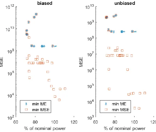
3.2.2. MSE minimization against ME minimization. ... 47
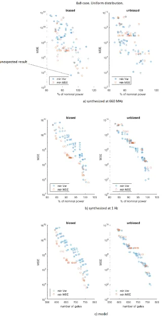
3.2.3. MSE minimization against variance minimization. ... 47
3.2.4. Leading M3 combinations against M2 combinations ... 50
3.2.5. Truncation of partial products against truncation of inputs... 51
3.2.6. DRUM ... 52
3.2.7. Low-power approximate MAC. ... 54
3.2.8. Approximate Booth multiplier against truncated Booth multiplier. ... 55
3.2.9. Truncation of partial products against other approximate techniques. ... 57
3.2.10. Effectiveness of using 2x2 multipliers. ... 61
3.2.11. Additional experiments for the 16x16 case. ... 64
3
4. Least-squares approximation applied to radio astronomy calibration. ... 67
4.1. Radio astronomy calibration. ... 67
4.2. Floating-point to fixed-point conversion. ... 69
4.3. Approximation of the Stefcal algorithm. ... 73
4.3.1. Truncation of partial products ... 75
4.3.2. Truncation of inputs ... 78
4.3.3. DRUM. ... 81
4.3.4. OR-compression. ... 82
4.4. Overview. ... 86
Conclusions. ... 87
Future work. ... 88
References. ... 89
4
Abstract.
5
Introduction.
Approximate computing is an emerging paradigm for the area, power and delay reduction. The reduc-tion of the power consumpreduc-tion is one of the main challenges in computing today, both for high-per-formance computing and for embedded systems. The core idea behind approximate computing is to simplify the logic of the circuit to achieve savings at the cost of accuracy reduction. Some applications are particularly tolerant to errors. These include audio and video applications as human end users are not able to notice small deviations, machine learning and artificial intelligence as these algorithms often can deal with erroneous data, digital signal processing as the real-world inputs are noisy. Many of these applications are resource-/power-hungry, and their error resilience can be exploited by using approximations to save energy, area, and increase performance at the cost of acceptable quality deg-radation.
Adders and multipliers are the main building blocks of computing units. In the recent years, many novel approximate adders and multipliers have been proposed in the literature. All of them introduce certain simplifications to circuits in order to decrease area, power, or critical path. The optimization of power and area is not something new, however. For example, when a floating-point algorithm needs to be mapped on hardware, it is desirable to use the fixed-point hardware as the logic circuits of fixed-point hardware are much simpler and the power consumption is smaller compared to those of floating-point hardware. In the process of mapping to fixed-point hardware, the main challenge is to optimize the bit widths of signals such that the total cost of the required hardware is minimized and at the same time the performance is satisfied. In this process the signals are truncated or rounded, introducing errors in the computation. In this case the arithmetic units stay accurate, but they operate on smaller signals. Also, to avoid the bit growth, truncated multipliers are often used in digital signal processing applications. The logic of these multipliers either stays accurate but the result is truncated, or the internal logic is simplified as well. These traditional methods can be thought of as belonging to the approximate computing domain as well, as they also enable a tradeoff between the accuracy and cost. In that sense, it is not clear what is the advantage of the new approximate computing methods in comparison to the traditional fixed-point truncation methods, as these new architectures are typi-cally not compared with the truncation methods.
One of the fields where the reduction of power is a critical challenge is the radio astronomy signal processing. An example is the upcoming Square Kilometer Array (SKA) which is going to have enor-mous power requirements. This array will have a large number of antennas, and each antenna ele-ment will receive noise dominated data. Approximate computing methods can be helpful in reducing the power consumption of the required computing units. One of the computations which can be ap-proximated is the calibration of antennas, which can be performed by iteratively solving linear least squares problems. In this work, the possibility of applying hardware approximate computing tech-niques to the least squares problem is investigated.
The research questions are formulated as follows.
- Comparison of various approximate computing techniques present in literature to investigate how the novel approximate methods perform compared to the traditional truncation meth-ods, and evaluation of their applicability to the least squares computation.
- Application of approximations to the radio astronomy calibration algorithm to determine how much energy can be saved by using different approximate computing methods.
6 multiplier-accumulator unit. Chapter 4 describes the application of the approximate methods to the radio astronomy calibration algorithm.
7
1. Literature review.
To efficiently apply approximate computing to a specific application, the error resilience of the appli-cation needs to be analyzed and an appropriate approximate computing technique should be chosen according to the error analysis. Error resilience analysis allows to identify instructions/kernels/data of a program where approximations could be allowed. Approximations then can be introduced by using software and hardware approximate computing techniques. In this chapter various error resilience analysis methodologies and different approximate computing techniques available in literature are considered.
1.1. Error resilience analysis.
Error resilience of applications can be attributed to several factors [9]:
• Noisy input – inputs from real world (from sensors for example) always contain some noise, and applications processing this data already know how to handle that noise. Errors intro-duced by approximate techniques can be regarded as additional noise.
• Redundant input data.
• Perceptual limitations – an image processing application can produce an image which contains some errors, but they are hardly noticed by a human user.
• Statistical, self-healing computation patterns – applications may employ computation pat-terns (such as statistical aggregation and iterative refinement) which intrinsically attenuate or correct errors.
• range of outputs are equivalent – i.e. no unique golden output exists
To effectively apply approximate computing, it is important to analyze error resilience of applications. An application always contains error-tolerant parts and error-sensitive parts. The goal of error resili-ence analysis is to identify the error-tolerant parts and the amount of approximations which can be applied on them, as well as to get insights into what kind of approximation techniques can be used. On the other hand, error-sensitive parts must be kept accurate as they include pointer arithmetic, conditions, control instructions – all these can lead to crashes and unacceptable results if they are approximated.
8 Analysis and Characterization of Inherent Application Resilience for Approximate Computing.
Chippa et al. [9] propose a systematic framework for Application Resilience Characterization (ARC). This framework partitions an application into resilient and sensitive parts and characterizes the resili-ent parts using approximation models that abstract a wide range of approximate computing tech-niques. The error resilience analysis is divided into three steps:
1) Profiling – distinguish dominant kernels. Kernels which run for more than 1% of the applica-tion overall time are chosen for analysis. Other kernels are considered to be not promising for approximations as they constitute only a small fraction of computations.
2) Identify error resilience – random errors are injected to the outputs of the dominant kernels and the overall output is checked against a relaxed quality function. This step is needed to partition kernels into sensitive and resilient. The error model is simple in this case (just random bitflips) and the quality function is relaxed.
3) Characterize error resilience – resilient kernels are analyzed by introducing errors according to the statistical approximation model (SAM) or according to a technique-specific approxima-tion model (TSAM). The result is validated with the actual quality funcapproxima-tion provided by the user.
As can be seen, steps 2 and 3 are identical. However, step 2 uses a simple error injection model and a relaxed quality function as this step is only needed to identify potentially resilient kernels and drop the ones which are clearly not appropriate for approximations.
The detailed analysis of the chosen kernels is performed in step 3. In that step errors are introduced according to the statistical approximation model (SAM) or a technique-specific approximation model (TSAM). SAM injects errors from a normal distribution based on three parameters: EM (error mean), EP (error predictability) and ER (error rate). This is a high-level approximation model as it does not represent any specific approximation technique, but rather indicates the amount of possible approxi-mations which can be applied to the analyzed computation. For example, such analysis can show that the application is tolerant to an error in some computation, with EM=0, EP=0.1, ER=1, which would mean that the computation output can have deviations of +-10% from its exact result and the appli-cation would produce acceptable output (according to the defined quality function). On the other hand, TSAM introduces errors in a more specific way. For example, it can introduce errors based on characteristics of some specific approximate adder according to its bit-error profile. Or it can model effects of bit truncation. On the algorithm level, it can skip some iterations in a loop, which corre-sponds to a software approximate technique called loop perforation.
9 Improving Error Resilience Analysis Methodology of Iterative Workloads for Approximate Compu-ting.
Gillani et al. [4] improved the ARC framework described above by introducing adaptive statistical ap-proximation model (ASAM). In addition to the original three parameters of SAM, namely error mean (EM), error predictability (EP) and error rate (ER), they use a new parameter, number of approximate iterations (NAI). The model allows to divide an iterative workload into exact and approximate itera-tions. They apply ASAM to a radio astronomy application and show that the approximation space ob-tained by ASAM is significantly larger than that of SAM. For this application, they show that the first 23% of iterations can be made approximate with certain EM, EP, ER, while the remaining iterations must be accurate. This allows to better exploit accuracy configurable and heterogeneous architec-tures, as approximate iterations can be assigned to inexact cores/modes, while sensitive iterations to exact counterparts. They also demonstrate that the original quality function may become inadequate in the error resilience analysis procedure, which requires defining an additional quality function to serve the purpose.
Quality of Service Profiling.
Misailovic et al. [5] introduce a quality of service (QoS) profiler which allows to identify sub-computa-tions that can be replaced with less accurate sub-computasub-computa-tions which deliver increased performance with acceptable quality of service loss. The profiler uses loop perforation (which transforms loops to perform fewer iterations than the original loop) to obtain implementations with different perfor-mance and quality of service characteristics. Sub-computations that consume a significant amount of computation time, demonstrate tolerance to loop perforation with acceptable QoS loss, and show significant increase in performance can be regarded as the best optimization targets. Such computa-tions can be perforated to increase performance, or they can be replaced by other optimized compu-tations. They argue that optimizable computations often contain loops that perform extra iterations, and that removing iterations, then observing the resulting effect on the quality of service, is an effec-tive way to identify such optimizable sub-computations. To quantify the quality of service, the profiler works with a developer-provided quality of service metric. They apply the profiler to a number of applications and show that loop perforation can increase the performance by a factor of between two or three (the perforated applications run between two and three times faster than the original appli-cations) with quality degradation of less than 10%.
iACT: A Software-Hardware Framework for Understanding the Scope of Approximate Computing. Mishra et al. [6] present iACT (Intel’s Approximate Computing Toolkit). It allows to analyze and study
the scope of approximations in applications. The toolkit allows to apply three approximate computing techniques: precision reduction, noisy ALU and memoization. The key idea is when the programmer writes a program, he/she annotates the approximation amenable functions (code segments) with high-level pragmas and also provides a quality function.
10 axc_precision_reduce – downconverts all the floating-point values in the function to 16-bit width pre-cision.
pragma axc_memoize – the tool creates a table with inputs and outputs of an approximated function. If during the execution the input values are within specified range with table inputs, then the result is read from the table skipping the function computation. Otherwise, the function is executed, and in-put/output values are written into the table.
As an example on how to use this toolkit, they include three different applications and analyze the scope of approximate computing in them. Applying precision reduction to a bodytracking application provides 22% dynamic energy reduction with less than 4% quality degradation. With the approximate memoization scheme applied to a Sobel filter, they obtain dynamic energy savings of up to 22% with 10% quality degradation. Finally, the effect of random bit failures is shown on the accuracy of a clas-sification algorithm. Random bit failures are representative of the timing failures which can happen at low-voltage or high-frequency operation modes. They show that even at high probability of these fail-ures (up to 0.5) the quality degradation is less than 5%.
ASAC: Automatic Sensitivity Analysis for Approximate Computing.
Roy et al. [7] propose ASAC – a framework which automatically identifies approximable data in an application. The main component of this framework is a specialized sensitivity analysis using statistical methods. Variables are systematically perturbed, and the output sensitivity is observed. A hypothesis
test generates scores for each variable to quantify the variable’s contribution to the output of the
program. Based on the scores, variables are classified as approximable or non-approximable. ASAC achieves 86% accuracy when compared to a manual annotation, which shows that this method can be used for large programs where a manual annotation is infeasible.
They evaluate their method by applying it to several benchmark applications. After identifying approx-imable variables, they apply bit-flip errors (by choosing a random bit among 16 lower bits and toggling it) to these variables and demonstrate that the applications are indeed amenable to the approxima-tions of these variables at the cost of acceptable quality degradation. For example, when bit-flip errors are injected to all the approximable variables in an FFT application, the QoS loss is around 3%. On the other hand, when they apply bit-flip errors to non-approximable variables, the output becomes unac-ceptable or the applications crash.
PAC: Program Analysis for Approximation-aware Compilation.
11 In comparison with ASAC, PAC demonstrates a more conservative behavior, i.e. some of the variables identified as approximable by ASAC are classified as non-approximable by PAC. The main advantage of PAC is the runtime overhead of the analysis – PAC is 3 orders of magnitude faster than ASAC. They evaluate PAC in a similar way as ASAC, by injecting bit-flip errors to approximable variables in a num-ber of applications. On average, about one third of the variables in the tested applications are classi-fied as approximable (they assumed that variables with DoA less than 0.5 are approximable and the rest are not). Applying bit-flip errors to these variables causes the QoS loss of 3.4% on average.
Error Resilience Analysis for Systematically Employing Approximate Computing in Convolutional Neu-ral Networks.
Hanif et al. [10] address the question of how to systematically employ approximate computing in Con-volution Neural Networks (CNNs). They divide the error resilience analysis into hardware level and software level analysis. There are two possible hardware approximation techniques that can be used for improving the efficiency of CNNs, quantization (floating point operations are transformed to fixed point and the word sizes of the activations and weights are reduced) and approximate hardware com-ponents (adders, multipliers, memory units). They argue that in both cases errors are introduced at multiple locations in a network and therefore the error resilience of a network can be simulated by introducing Random Gaussian or White Gaussian Noise (RGN or WGN) at particular locations in a net-work (because errors from multiple sources, when added together, generate a Gaussian distribution). They introduce WGN individually at the output of convolutional layers and observe the effects on the output accuracy of the network. They apply this analysis to an image classification network and show that the network has a different level of error tolerance for the same error in different convolutional layers. For the software level analysis, they propose a technique which computes the significance of a filter in a layer. Filters with low significance can be pruned at the cost of low quality loss.
Algorithmic-level Approximate Computing Applied to Energy Efficient HEVC Decoding.
12
1.2. Approximate computing techniques.
Approximate computing techniques can be broadly divided into software techniques and hardware techniques.
Software techniques:
• computation skipping – some computations are skipped at the cost of acceptable quality loss. Examples include loop perforation, filter pruning, memoization, reducing the number of iter-ations of an iterative process.
• computation approximation – computations can be replaced by less complex approximate al-ternatives with lower accuracy. For example, the order of a filter can be reduced, or a Finite Impulse Response (FIR) filter can be replaced by an Infinite Impulse Response (IIR) filter [11]. Hardware techniques:
• circuit pruning – combinational logic can be made simpler by reducing the number of logic gates at the cost of introducing errors. For example, arithmetic elementary circuits such as full adder and 2x2 multiplier can be made smaller at the cost of making some of the entries in their truth tables to be erroneous.
• Data sizing – usage of less accurate data representation to reduce the complexity of arithmetic operations and storage requirements. For example, fixed-point representation with optimal bit-width satisfying quality requirements can be used instead of floating point numbers. An-other example is quantization – 32-bit result of multiplying two 16-bit numbers can be trun-cated or rounded to 16 bits for further processing in the datapath.
• Voltage overscaling – the supply voltage is reduced to the point at which occasional timing errors occur and the circuit starts producing errors. These timing errors affect critical paths which are usually involved in the computation of the most significant bits, which means that voltage overscaling is likely to lead to large errors. This makes it hard to achieve smooth deg-radation in accuracy as voltage decreases. It can also be hard to predict which errors will be produced at which voltages, as this can depend on a lot of factors such as layout and manu-facturing process.
In this section circuit pruning and data sizing are considered and some of the important work done in this area is discussed.
Low-Power Approximate MAC Unit.
Esposito et al. [1] present a low-power approximate multiply-accumulate unit. They keep the accumu-late part (adder) accurate and approximate the partial product matrix (PPM) using two methods:
• Approximate counters – if there are two partial products x2y8 and x8y2 in a column, their sum x2y8 + x8y2 can be approximated by the OR-gate: x2y8 OR x8y2. So, two partial products are reduced into a single term. In this case only one input pattern out of 16 produces an error. When x2=x8=y2=y8=1 the correct sum is 2, while the OR-gate produces result 1 in this case. If the height (the column with maximum number of partial products) of the original PPM is N, this approach allows to halve the PPM height making in N/2 by using OR-gates in the columns which have height larger than N.
13 They also compute the error introduced by the column deletion and approximate compression and improve the MAC accuracy by initializing the accumulation register with a compensation term equal to the computed mean error multiplied by the number of multiplications. The proposed MAC units with different configurations show area and power improvements ranging, respectively, from 39% to 69% and 40% to 71%. They also use their MAC in an image filtering application and show significant power reduction with tolerable image quality degradation.
Approximate 1-bit full-adders.
Several papers describe approximate 1-bit adders [2] [3] [15]. In these works, the logic of full-adders is simplified at the cost of introducing errors in the truth tables. These full-adders differ in the number of logic gates they use and in error patterns they introduce (number of erroneous outputs, magnitudes of errors).
Approximate 2x2 multipliers.
Kulkarni et al. [17] present an underdesigned multiplier architecture which consists of approximate elementary 2x2 multiplier blocks that generate partial products. The 2x2 multiplier produces only 1 error when all four inputs are 1 (3x3 is equal to 7). Rehman et al. [2] describe other 2x2 multiplier designs with different structures and various error characteristics (error magnitudes, error probabili-ties).
Architectural-Space Exploration of Approximate Multipliers.
Rehman et al. [2] propose a methodology to generate and explore the architectural space exploration of large-sized multipliers using the following design parameters:
• different types of elementary approximate 2x2 multiplier modules
• different types of elementary 1-bit full adder modules for summing the partial products
• selection of bits for approximation – how many LSBs need to be approximated in the adder tree?
The design space grows very fast with the width of the operands. They show that even for the 4x4 multiplier, there are 7500 possible configurations. They propose a depth-first search algorithm which starts using the highest approximation available and moves towards a more accurate solution. It stops at a certain configuration (of adder, multiplier and bit-width) when the provided quality function is satisfied. They apply a subset of design points to a JPEG application and show corresponding power/area/quality results.
Approximate multipliers for MAC.
14 adds to the design space a multiplier with 3x3=11 entry. By using different combinations of 2x2
mul-tipliers it’s possible to construct a multiplier with the mean error close to zero. The output of the whole
multiply-accumulate unit will also have zero-mean error. Using an exhaustive search algorithm, he finds a configuration with the best quality for a cost constraint, or a configuration with the lowest cost for a quality constraint.
DRUM: A Dynamic Range Unbiased Multiplier for Approximate Applications.
Hashemi et al. [18] propose a novel approximate multiplier with a dynamic range selection scheme and an unbiased error distribution. The main idea of their method is to use an exact multiplier but with smaller operand widths. If the operands to multiply have width n, they use a kxk-bit multiplier (k<n) and choose the k bits from each operand by detecting the leading 1 in the bit pattern and select-ing k bits startselect-ing from there. It means that instead of approximatselect-ing the multiplication process, they approximate the operands while using an exact multiplier. The 2k-bit result is then shifted to the left by a certain number of bits depending on the positions of the leading ones in the original operands to get a 2n-bit result, while placing zeros at the least-significant bits. To make the truncation error to have near-zero mean when selecting k bits from the operands, 1 is always placed at the least-signifi-cant bit of the newly formed k-bit operand. This allows the multiplier to be unbiased and have a near-zero average error. As a result, when using this multiplier in real applications involving numerous mul-tiplications some errors potentially cancel each other rather than accumulate in the final result of the computation.
They compare their multiplier with other two approximate multipliers including [17] in stand-alone manner as well as in three different applications from the domains of computer vision, image pro-cessing and data classification, and demonstrate a better overall power/quality tradeoff of the DRUM.
The Hidden Cost of Functional Approximation Against Careful Data Sizing.
15
2. Multiply-accumulate unit and its approximation.
2.1. Least Squares Problem
Least squares is a method of finding approximate solutions of over-determined systems of linear equa-tions [31]. Over-determined systems are systems with more equaequa-tions than unknowns. Consider a system of linear equations 𝐴𝑥 = 𝑏 with an 𝑚𝑥𝑛 matrix 𝐴 (𝑚 > 𝑛 as it’s overdetermined), 𝑛-vector 𝑥, and 𝑚-vector 𝑏. Such a system has a solution only if 𝑏 is a linear combination of the columns of 𝐴. If a solution does not exist, i.e., there is no such 𝑥 that satisfies 𝐴𝑥 = 𝑏, it is possible to find a vector 𝑥 that minimizes the error vector 𝑟 = 𝐴𝑥 − 𝑏 which is called the residual vector. In this case 𝑥 almost satisfies the linear equations and 𝐴𝑥 ≈ 𝑏. Minimizing the residual vector means making its length as small as possible. The length of a vector is given by its norm which is equal to the square root of the sum of the squares of its elements:
‖𝑟‖ = ‖𝐴𝑥 − 𝑏‖ = √𝑟12+ 𝑟
22+ ⋯ + 𝑟𝑚2 (1)
The problem of minimizing the norm ‖𝑟‖ is the same as the problem of minimizing the square of the norm ‖𝑟‖2= 𝑟
12+ 𝑟22+ ⋯ + 𝑟𝑚2. The least squares problem therefore can be formulated as follows: min
𝑥 ‖𝐴𝑥 − 𝑏‖
2 (2)
If the columns of 𝐴 are linearly independent, the solution of the least squares problem is given by:
𝑥 = (𝐴𝑇𝐴)−1𝐴𝑇𝑏 (3)
If 𝐴 is a vector instead of a matrix and denoted as 𝑎, the least squares problem is reduced to finding a scaling 𝑥 which makes 𝑎𝑥 as close as possible to 𝑏. The solution 𝑥 is computed by dividing the dot product of 𝑎 and 𝑏 by the dot-product of 𝑎 with itself:
𝑥 = 𝑎
𝑇𝑏
𝑎𝑇𝑎 (4)
This problem can also be formulated as the problem of finding the projection of 𝑏 onto 𝑎. An example for two-dimensional vectors is shown in Fig. 1. The goal is to find a scaling factor 𝑥 such that 𝑎𝑥 is a projection of 𝑏 onto vector 𝑎. In this case vector 𝑎𝑥 has the smallest possible distance from 𝑏 among all vectors with the same direction as 𝑎 as 𝑟 = 𝑎𝑥 − 𝑏 is perpendicular to the direction of vector 𝑎. If 𝑎 = (1, 2) and 𝑏 = (8, 3), the scaling is computed as follows: 𝑥 = 𝑎𝑇𝑏
𝑎𝑇𝑎= 1∙8+2∙3
12+22 = 2.8.
16
Figure 1. Least squares problem in a simple case with two vectors.
2.2. Multiplier-accumulator (MAC)
MAC and SAC are the most computation-intensive units of the least squares computation. The vectors in applications can be very large, consisting of hundreds or thousands of elements and the computa-tion of the two dot-products is the dominant part of the least squares algorithm. Division is done only once at the end of the computation when the numerator and denominator are known. For this reason, in this work the division unit is assumed to be accurate as approximating it would produce a large error for a minimal reduction in cost. By cost, the area, power or latency of a circuit is meant. As the SAC is a special case of the MAC with simplified logic due to the equal operands, this section describes a more general MAC unit, but the discussion is relevant to the SAC as well.
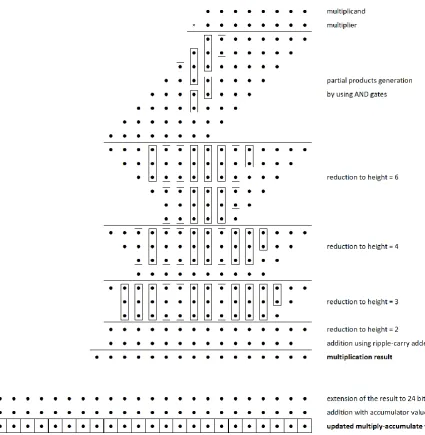
A multiplier-accumulator consists of a multiplier, an adder, and registers which store an intermediate result. All three can be made approximate by using approximate multipliers, adders, or approximate storage techniques. However, the multiplier part typically has the largest cost in terms of hardware and power required, which makes it the first target for approximation attempts and the focus of this work. An example of an accurate 8x8 MAC unit in dot notation (similar to [20]) can be seen in Fig. 4. The operation of a MAC unit can be divided into five stages:
1. Partial products generation – in Fig. 3 the partial products are generated by 64 AND gates. Each row of the partial product matrix represents the multiplicand value multiplied by 0 or 1 depending on the multiplier bit. This value is also shifted such that the least significant bit (LSB) has the same position as the multiplier bit. In this case each row is either 0 or 1𝑎 and there are 𝑛 rows for an 𝑛𝑥𝑛 multiplier. If the modified Booth algorithm is used, the number of rows is half as much, 𝑛/2, as each row can represent 0, ±1𝑎, ±2𝑎. In case of a squarer such matrix is significantly simplified as some of the AND gates have equal inputs, allowing to significantly reduce the number of rows [20].
17 reduce the matrix: Wallace tree and Dadda tree. In the Wallace method, the partial products are reduced as soon as possible, and in the Dadda tree the reduction is done by using the smallest possible number of adders to reduce the height to the next optimal value (for an 8x8 case, these values are 6-4-3-2). The Dadda tree is slightly faster and requires fewer gates [21]. In Fig. 4 the Dadda method is used. The height is reduced from 8 to 2 in four stages: 8-6-4-3-2. The Dadda method is also used to estimate the cost of various designs later in the work. 3. Addition after reduction – the resulting two operands are then added by a carry-propagate
adder to produce the final multiplication result. It can be a simple ripple-carry adder in which case the addition after the reduction can be seen as continuation of the partial products re-duction as it is done by using half adders and full adders to reduce the height from two to one. But this addition can also be done by using a faster adder, for example the carry-lookahead adder.
4. Accumulation – the multiplication result is extended and added to the running sum which is stored in the accumulator registers. The accumulator has a larger bit width as it has to store the sum of a large number of multiplications. The size is chosen depending on the number of elements in the vectors and the distributions of their values to avoid an overflow.
5. Storing the result – the multiply-accumulate value is stored into registers and the process is repeated for the next pair of inputs.
Figure 2. Operation of full adders and half adders.
18
Figure 4. Dot diagram of an 8x8 MAC unit.
2.3. Unit gate model
In this work a simple unit gate model [22] is used to estimate the area of various designs and make comparisons. In this model the NOT gate is equal to 0.5 gates, two-input gates AND, OR, NAND, NOR are assigned a value of 1, and the XOR gate has a cost of 2 gates. Areas of some other components according to this model are shown in Table 1.
Component Area in gates
NOT 0.5
AND, OR, NAND, NOR 1
XOR 2
Full adder 7
Half adder 3
[image:19.595.96.522.65.501.2]Register (master–slave D flip-flop) 9
19 Table 2 shows the results of applying this simple model to the MAC unit. As can be seen, the multiplier part (the first three stages) has more area than the accumulation and registers combined. However, these values depend on the architectures of the components (in this case, for example, the adder is assumed to be a ripple-carry adder). Also, the sizes of the accumulation stage and registers can be made smaller or larger depending on the overflow behavior.
MAC stage Area in gates Percent of total area
Partial products generation 64 8%
Partial products reduction 266 33%
Addition after reduction 94 12%
Accumulation 164 20%
Storing the result 216 27%
Table 2. Area of MAC computed using simple gate model.
2.4. Errors and error metrics.
20
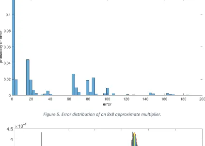
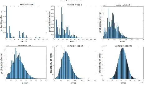
[image:21.595.86.510.83.384.2]Figure 5. Error distribution of an 8x8 approximate multiplier.
Figure 6. Error distribution of a MAC with an approximate 8x8 multiplier.
21
Figure 7. MAC error distribution as the size of vectors increases.
To quantify the error distribution at the output of the MAC the position of the distribution and the width of the distribution must be considered. The position can be described by the distance from 0 to the center of the distribution, which is equal to the mean error (ME), i.e., sum of errors divided by the number of outputs.
𝑀𝐸𝑚𝑎𝑐 =
1 𝐾∑ 𝑒𝑖
𝐾
𝑖=1
(5)
where 𝐾 is the number of MAC results (𝐾 = 100000 in Fig. 5) and 𝑒𝑖 is the error of an individual MAC result. The simplest way to describe the width is to measure the distances from the mean to the far-thest errors to the left and right of the mean, the maximum deviation. However, this measure depends only on the extreme values and does not reflect the fact that typically these extreme errors are rare and most of the errors are gathered around the mean value. There are many error combinations which lead to the mean error and there are only few combinations producing large errors. A more reliable measure of the width of a distribution that depends on all errors is the standard deviation 𝜎:
𝜎𝑚𝑎𝑐= √ 1
𝐾∑(𝑒𝑖− 𝑀𝐸𝑚𝑎𝑐) 2 𝐾
𝑖=1
22 Sometimes it is more convenient to use the square of the standard deviation, the variance, as a measure of the distribution width:
𝑉𝑎𝑟𝑚𝑎𝑐= 1
𝐾∑(𝑒𝑖− 𝑀𝐸𝑚𝑎𝑐) 2 𝐾
𝑖=1
(7)
The mean error or variance alone are not sufficient to describe errors. If only the mean error is used, there is no information about the spread of the errors from the average error. It may be that the mean error is equal to 0, but the spread is large, and the error becomes significant. It means that it’s not
possible to conclude that one approximate design is better than another just by comparing the mean errors. Similarly, if the variance is close to 0, but the distribution is far from 0, i.e., the mean error is large, the total error will also be significant. Therefore, the variance alone cannot be used to compare approximate MAC designs either.
Error metrics exist which combine the position and width of an error distribution into a single value [23]. An example is the widely used mean squared error (MSE).
𝑀𝑆𝐸𝑚𝑎𝑐 = 1
𝐾∑(𝑒𝑖) 2 𝐾
𝑖=1
= 𝑀𝐸𝑚𝑎𝑐2 + 𝑉𝑎𝑟𝑚𝑎𝑐 (8)
It incorporates both the mean error and the variance and thus can be used to compare approximate MAC designs. However, it is not possible to compute ME and variance if only the MSE number is given. This fact makes it hard to use the MSE metric to understand the origin of the errors, i.e., are the errors coming from a large mean error or a large variance? The answer to this question determines error mitigation possibilities as will be described in the next section.
The mean absolute error (MAE) is similar to MSE [23]. It also combines the position and width of an error distribution and can be used for comparisons. The difference is that in the MSE metric larger errors have more weight as they are squared.
𝑀𝐴𝐸𝑚𝑎𝑐= 1 𝐾∑|𝑒𝑖|
𝐾
𝑖=1
(9)
Fig. 6 contains information about the magnitudes and signs of errors between accurate and approxi-mate MAC results. There is no information about the relative errors. For example, if there are two accurate outputs of MAC which are equal to 5 and 105, and two corresponding approximate results 10 and 110, in both cases these errors will be plotted as -5 on an error histogram similar to Fig 6. However, in the first case there is a percentage error of 100 ∙ (10 − 5)/5 = 100%, while in the sec-ond case it’s only 4.76%. To quantify this relative error at the output of the MAC the mean absolute percentage error (MAPE) can be used [23]. The main disadvantage of this metric is that if the exact result is zero, it’s undefined, which makes it difficult to use this metric for signed numbers.
𝑀𝐴𝑃𝐸𝑚𝑎𝑐 = 100
𝐾 ∑ |
𝑒𝑖 𝑒𝑥𝑎𝑐𝑡 𝑟𝑒𝑠𝑢𝑙𝑡| 𝐾
𝑖=1
(10)
23
2.5. Mitigation of errors.
The concepts of the mean error and variance described in the previous section can be used to under-stand what can be done to reduce the errors at the output of a MAC unit. If an exact multiplier is used, the bias is zero and variance is also zero, which corresponds to the straight vertical line at zero in Fig. 6. If an approximate multiplier is used, a certain bias and variance are introduced at the output of the MAC which depend on the input distribution, error profile of the multiplier and the size of the vectors.
2.5.1. Mean error balancing.
The first approach is to make the mean error of the approximate multiplier to be zero for a given distribution. If the expected error of the multiplier is zero, the expected error of the MAC will also be zero as the expected value of a sum is equal to the sum of expected values of individual variables (multiplier errors in this case).
𝑀𝐸𝑚𝑎𝑐 = 𝑁 ∙ 𝑀𝐸𝑚𝑢𝑙𝑡 (11)
where 𝑁 is the number of multiplications needed to compute the dot-product, i.e., the vector size. This approach can only be used by certain approximate computing techniques which allow such mean error balancing. For example, this method can be used in recursive multipliers which consist of smaller 2x2 elementary multipliers (described in a later section). By using a certain combination of 2x2 multi-pliers with different positive and negative errors the mean error can be made smaller. This method is considered in [12]. The main advantage is that in theory the vector size is not important because if the mean error is 0, addition of any number of multiplier results will produce the expected mean error of zero at the output of the MAC unit. In practice, however, it is often not possible to find a combination with mean error exactly equal to zero as there are a limited number of possible approximate 2x2 de-signs and their combinations. Therefore, the mean error will be non-zero and the bias at the MAC output will be farther and farther away from zero as the length of the vectors grows.
Another problem is that this approach ignores the variance. Low mean error does not guarantee any-thing about the error behavior at the MAC output, it only says that the distribution is centered at zero, but the width of it is unknown. It is therefore impossible to predict the MSE or other error metrics which take into account both the width and bias of the distribution. The MSE of a MAC can be com-puted using the mean error and variance of the multiplier as follows:
𝑀𝑆𝐸𝑚𝑎𝑐 = 𝑀𝐸𝑚𝑎𝑐2 + 𝑉𝑎𝑟𝑚𝑎𝑐= (𝑁 ∙ 𝑀𝐸𝑚𝑢𝑙𝑡)2+ 𝑁 ∙ 𝑉𝑎𝑟𝑚𝑢𝑙𝑡 (12)
Therefore, to minimize the MSE of a MAC, both the mean error and variance of the multiplier must be minimized. Mean error balancing, however, introduces a trade-off between the mean error and vari-ance. It might be that the mean error is minimized at the expense of increased varivari-ance. For example, a design with mean error zero can use more approximate 2x2 blocks than a design with non-zero mean error, which means that the variance of the zero mean error design is larger and that can lead to larger errors at the output of the MAC unit. Also, this approach is hardware oriented and if the input distri-bution is changed, the hardware must be changed as well to remove the bias.
2.5.2. Using two multipliers with opposite errors.
24 one multiplier is used for all multiplications, as the error profile of both multipliers is the same except the signs. This approach is described in [19]. The main advantage of this method is that the mean error is zero independent of the size of the vectors. Also, if the distribution is changed, the mean error will stay at zero as the mean error of one multiplier will be balanced by the opposite multiplier. The main disadvantage is that two multipliers are required, making this method inapplicable to area optimiza-tion. Also, it can be hard to design a multiplier with an error profile which is opposite of a given mul-tiplier and it can be less efficient in terms of error/cost tradeoff. In [19] the mirror mulmul-tiplier with +𝛿 bias always has larger area and power compared to the multiplier with −𝛿.
2.5.3. Accumulator initialization.
Another approach is to place a compensation initial value in the accumulator register, i.e., instead of starting with 0 inside the accumulator, the accumulation register is initialized with some predefined compensation value. This value is equal to the mean error of the multiplier, multiplied by the size of the vectors. The position of the distribution can be controlled by this initial offset and shifted to zero. This method can be used with any approximate multiplier as the unbiasing is done outside of the multiplier. Another advantage of this method is that the unbiasing value can be adjusted according to the current distribution and therefore it is not needed to change the hardware if the distribution is changed. The main disadvantage is that the size of the vectors must be known to compute the required compensation term. However, in most applications this size is known before the computation. Also, this compensation term is a constant which is added to all the results independent of the real values, which can lead to large errors in certain applications, especially if the distribution is not stable and changes frequently.
This method allows to optimize the MSE of the MAC unit, as the variance and the mean error in Eq. 12 can be minimized independently and therefore there is no tradeoff between the two. The multiplier part in this method is optimized to have the smallest possible variance without considering the mean error of the multiplier, as this mean error will be compensated in the accumulator. The mean error of the MAC will be zero after unbiasing. The variance will be equal to the variance of the multiplier times the number of multiplications if errors of individual multiplications are uncorrelated, as the variance of a sum of independent random variables is equal to the sum of the variances of these variables. If they are correlated, then the covariance between each pair of multiplications has to be computed and added to this sum. However, the sum of individual variances is a good approximation to the total MAC variance if this correlation is not large.
𝑉𝑎𝑟𝑚𝑎𝑐= 𝑁 ∙ 𝑉𝑎𝑟𝑚𝑢𝑙𝑡 (13)
25
2.6. Approximate units against careful data sizing.
The work of [14] have compared a number of approximate circuits with careful data sizing. By careful data sizing they mean the choosing of the right bit-widths for the signals. The results suggest that the benefits of using approximate functional units seem to be minimal or even nonexistent for the con-sidered set of real-world applications. One of the researchers in the field even claims that it is a closed problem in the approximate computing research and we should stop designing approximate circuits because exact units with a narrower bit width are at least as good as approximate ones [24].
Choosing a smaller bit-width for a functional unit introduces an error due to truncation, but it has a positive impact on the functional units which use the output as they also can be made smaller. Ap-proximate functional units, on the other hand, have the same number of output bits as their accurate counterparts. The hardware cost of the particular unit can be decreased by introducing errors and simplifying its logic, but the subsequent units which are using the computed approximate result still have to operate on the same bit-widths.
It seems that if the datapath after the approximated unit is long enough, it is always better to use truncation (smaller bit-widths). To illustrate this, suppose that a multiplier is approximated. If an ap-proximation technique is used which does not reduce the number of output bits, the cost is saved only in the multiplier itself but not in the subsequent circuits as the output bit-width is not changed. The error is propagated, and the exact units spend energy and area processing erroneous data. On the other hand, if a multiplier is approximated in such a way that some of its least-significant bits are always zero, it may save less cost in the multiplier, but these zeros are propagated to the whole datapath, including registers, adders, other multipliers, multiplexers and so on. If this datapath is long enough (an IIR/FIR filter, for example), the benefits will outweigh the savings in just one multiplier. Errors from the truncated unit are also propagated to the datapath, but the cost is saved as the sub-sequent units are also truncated, so the errors are propagated in the form of truncation.
Some of the units after an approximated unit can also be made approximate by introducing more errors on top of the already propagated errors, but not all circuits are easily approximable (consider registers or multiplexers as an example) and the nets and buses between the units cannot be simpli-fied. Also, the error profile in such a multi-level approximation scheme can be more difficult to analyze and predict than truncation. Another possibility is to truncate the output of an approximate unit. In this case two types of approximation are used – the approximate result with an introduced error has the same number of bits as the accurate one, but then only some of the computed bits are used by the subsequent units.
These issues seem to be the main limitation of approximate functional units and it is not considered in many papers proposing such units. Typically, approximate adders and multipliers are evaluated in isolation and there is no comparison with the simplest approximation – truncation. Such units are compared with their accurate counterparts and the achieved cost/error trade-off is reported. How-ever, it may be that a similar or even better tradeoff can be achieved simply by using truncation tech-niques.
26
2.7. Approximate multipliers for MAC.
In this section several techniques for approximating a multiplier are described. The selected tech-niques have different approximation principles and their comparison with truncation should help to understand their effectiveness compared to truncation methods.
2.7.1. Recursive approximate multipliers
Recursive multipliers are multipliers consisting of 2x2 elementary multipliers. It is a hard task to design an arbitrary 𝑛𝑥𝑛 approximate multiplier, but a 2x2 multiplier is a simple circuit which can be made approximate by removing some gates and modifying its truth table. These small multipliers can be used as building blocks for larger multipliers. Several approximate 2x2 designs are available in the literature with various error and cost properties. A combination of accurate and different approximate 2x2 blocks can be used to construct approximate multipliers with certain error properties based on a given input distribution.
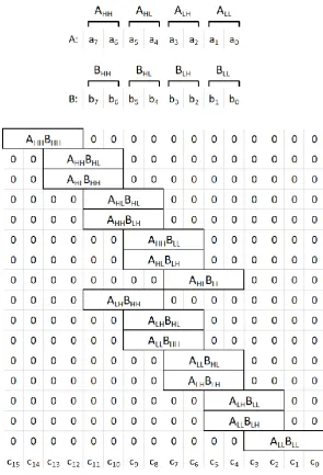
Five 2x2 designs are considered, one accurate and four approximate (Fig. 8). Approximate designs are smaller than the accurate one in terms of cost, but they introduce various errors which can be seen in the corresponding truth tables. An example of an 8x8 multiplier consisting of sixteen 2x2 multipliers can be seen in Fig. 9. The mean errors and variances (assuming uniform distribution) of the multipliers are shown in Table 3. As the errors are of different magnitudes, signs and frequencies, these elemen-tary 2x2 blocks can be combined to achieve the best cost-error trade-off for a given input distribution. Different ways of combining these 2x2 blocks are considered next.
27 2x2 type Mean error Variance
M1 -0.1875 0.15234375
M2 -0.125 0.234375
M3 0.125 0.234375
[image:28.595.211.388.73.134.2]M4 -0.25 0.9375
Table 3. Mean error and variance of 2x2 multipliers assuming uniform distribution.
Figure 9. 8x8 multiplier consisting of 2x2 multipliers [12].
Low mean-error combinations:
[image:28.595.147.443.179.613.2]28 Another disadvantage is that for finding the best design for a given cost (generation of the trade-off) an exhaustive search over a large design space is required. It is feasible for 4x4 multipliers, as the design space includes only 54 = 625 combinations (the accurate design plus four approximate de-signs, raised to the power which is equal to the number of required 2x2 blocks, four in this case). But the design space grows exponentially with the multiplier size. For an 8x8 multiplier consisting of 16 2x2 multipliers, there are 516= 152,587,890,625 possible combinations. For this reason, exhaustive search is only used for 4x4 multiplier tradeoff generation. For 8x8 case, the design is partitioned into four 4x4 multipliers. For each of these four multipliers a separate tradeoff is generated considering all 625 possibilities, from which only 60 pareto-optimal and close-to-pareto-optimal combinations are taken. This leads to 604 = 12,960,000 combinations from which the final tradeoff is generated. The approach for the tradeoff generation for an 8x8 multiplier can be described as follows:
1. Construct multipliers consisting exclusively of a certain type, M2 for example. Measure the power and area of the multiplier and divide it by the number of 2x2 blocks (16 in the 8x8 case). This way a certain weight is assigned for each type. Typically, M0 has the largest weight as it’s
accurate, and M2 has the smallest weight.
2. For each of the four 4x4 multipliers compute the cost (based on the determined weights) and the error according to an error function (ME, MSE, or variance) and the given input distribu-tion. This way each of the 625 combinations is assigned a cost and an error.
3. Select a number of Pareto-optimal designs from each of the 4x4 tradeoffs, 60 for example. The larger the number, the more optimal the tradeoff, but the complexity of the search is also increased.
4. Merge all the selected combinations and find the best designs.
This approach is used for finding the best designs among the low mean-error combinations, and in each of the combinations considered next as well, except those which consist of only one type where the tradeoff generation is trivial.
Low variance combinations (not including covariance):
The variance of a multiplier can be computed by summing the variances of all 2x2 multipliers and covariances between each pair of the blocks:
𝑉𝑎𝑟(𝑚𝑢𝑙) = 𝑉𝑎𝑟(𝑚𝑢𝑙1) + 𝑉𝑎𝑟(𝑚𝑢𝑙2) + ⋯ + 𝑉𝑎𝑟(𝑚𝑢𝑙𝑛) + 2 ∑ 𝐶𝑜𝑣𝑎𝑟(𝑚𝑢𝑙𝑖, 𝑚𝑢𝑙𝑗) 𝑖≠𝑗
(14)
29 information about the variance in the ME metric. The low variance approach with unbiasing, however, allows to minimize the width of the error distribution and then shift it to zero with unbiasing to mini-mize errors.
This method only uses combinations with the M1 and M2 multiplier types. The M3 type is not useful for such combinations because it has the same variance as M2, but higher cost, so M2 is always better to use (if covariance is ignored). M4 is always worse than M2 as they both have an error for the same 3x3 case, but the error of M4 is twice as large which means that it always has a larger variance. More-over, the area is also larger as M4 has an XOR-gate instead of an OR-gate in M2.
Low MSE combinations
These combinations minimize the MSE of the MAC unit by minimizing both the mean error and vari-ance in Eq. 12. For a 4x4 case, the MSE of each combination out of 625 is computed and the pareto-optimal combinations are selected. For an 8x8 case, similar to low mean error combinations, the de-sign is divided into four 4x4 blocks, the best 60 dede-signs are chosen to form a dede-sign space of 12,960,000 combinations, and then the pareto-optimal designs are included in the tradeoff. Contrary to the low-variance approach, this method introduces a tradeoff between the mean error and vari-ance. Therefore, all 2x2 multiplier designs are present in such combinations. It is expected that these combinations should produce a more effective tradeoff compared to low mean error and low variance combinations if the unbiasing is not performed, but low variance combinations with unbiasing should produce better results compared to low MSE with unbiasing.
M2 combinations
There is a significant difference between the M2 and M4 types and the two other approximate 2x2 multipliers. M2 and M4 produce only 3 bits as output, which means that there are fewer partial prod-ucts to add in the adder tree (Fig. 10). Therefore, these 2x2 blocks save cost at the partial product generation stage and also reduce the adder tree cost. M1 and M3, on the other hand, have 4 bits at the output, the same as the accurate type M0. When using M1 and M3, savings are made only in the partial product generation step. This issue is not considered in the papers which propose M1 [2] and M3 [19]. The partial product generation cost increases quadratically with the multiplier size, but the adder tree cost presumably grows faster. Table 4 shows the costs of partial products generation (num-ber of AND gates) and the costs of the required Dadda trees (num(num-ber of FAs and HAs) to sum them. If the unit gate model is used which counts a full adder as 7 gates and a half adder as 3 gates, the relative cost of the partial product generation decreases with the multiplier size. If these estimations reflect the real grow rate, the usage of M2 multipliers becomes more effective with larger multipliers com-pared to other elementary types.
Considering that M2 has the smallest area and it reduces the addition tree, it can be expected that this type is the most efficient 2x2 multiplier among the considered types. The only drawback is a larger variance compared to M1. The tradeoff is very simple as there is only one type. It starts with all blocks of the accurate type M0 and the next block with the smallest expected error is made approximate. This process is repeated until all the blocks are of the type M2.
30
Figure 10. Partial products produced by 2x2 multipliers when they are used in a 4x4 multiplier.
Multiplier size AND gates for partial prod-ucts
Full adders for Dadda tree
Half adders for Dadda tree
Dadda tree cost estimation in gates
Partial prod-ucts cost di-vided by Dadda tree cost
4x4 16 3 1 24 0.67
8x8 64 34 6 256 0.25
16x16 256 194 14 1400 0.18
32x32 1024 898 30 6376 0.16
64x64 4096 3842 62 27080 0.15
Table 4. Costs of partial products and Dadda trees for multipliers of different sizes according to the simple gate model.
M1 combinations
Combinations consisting of only M1 and M0 types are also included in the comparison as M1 has the lowest variance among the considered 2x2 multipliers (if the input distribution is uniform). M1, how-ever, does not have a positive impact on the compression tree, so it is expected that the M1-only approach is worse than the M2-only combinations. The tradeoff generation is the same as for M2.
Leading M3 combinations (covariance aware combinations)
In the low-variance approach, the covariance is ignored. If a design does not contain an M3 type mul-tiplier, the covariance can be ignored as in such combinations all the correlations are positive and the total variance is at least the sum of the individual variances, taking into account the covariance can only make the variance larger. If, however, there is an M3 type multiplier in the combination, it can reduce the variance. As an example, if there is an error in a 2x2 M2 type block, and there is an M3 block with shared inputs, when the M2 type has an error, there is a higher probability that the M3 type will also produce an error, but of the opposite sign, which can partially reduce the variance of such a combination compared to a combination consisting of only the M2 type.
As an example, Fig. 11 shows the combination M0-M0-M3-M2, which will be labeled as 0032 for short. The most significant block is accurate, M0, and the least significant block is of type M2. M3 and M2 blocks have a shared input 𝐴𝐿. If the covariance is ignored, the variance in case of the uniform distri-bution can be estimated as 𝑉𝑎𝑟(0032) ≈ 𝑉𝑎𝑟(𝑀2) + 𝑉𝑎𝑟(𝑀3) = 0.234375 + 16 ∙ 0.234375 = 3.984375. If the covariance is included, the variance can be computed precisely as 𝑉𝑎𝑟(0032) = 𝑉𝑎𝑟(𝑀2) + 𝑉𝑎𝑟(𝑀3) + 2 ∙ 𝐶𝑜𝑣𝑎𝑟(𝑀2, 𝑀3) = 0.234375 + 16 ∙ 0.234375 + 2 ∙
31 variance. If there is an error in M2, there is a high probability of partially cancelling this error by the M3 block.
Figure 11. 0032 combination.
In comparison, if the combination is 0022, the variance becomes larger. If there is an error in one block, there is a higher probability of error in another. The variance of this combination is increased by the covariance term: 𝑉𝑎𝑟(0022) = 0.234375 + 16 ∙ 0.234375 + 2 ∙ 0.1904296875 = 4.365234375. As can be seen, the covariance of the 0032 combination is smaller than of the 0022 combination. However, M3 is less effective compared to M2. To understand the impact of this effect, combinations consisting of M3 type at the most significant block followed by M2 blocks are also in-cluded in the comparison.
Truncation of partial products
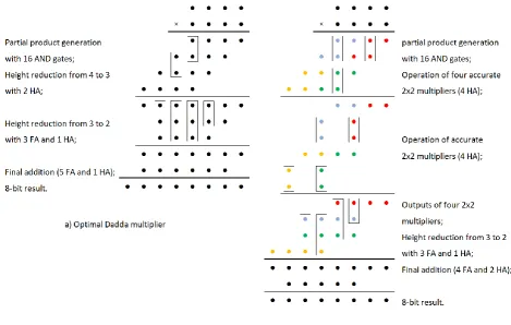
Truncation of partial products is normally done by removing AND gates (Fig. 12). If this approach is used here, however, it will lead to a slightly different architecture compared to the recursive multipli-ers. Recursive multipliers use small 2x2 multipliers to produce four partial products. Essentially an accurate 2x2 multiplier compresses the four AND gates with two half adders such that the results have the height of one (Fig. 13a). The four AND gates can be seen in the scheme of the accurate 2x2 multi-plier (Fig. 8). The two half adders can also be recognized there. One half adder consists of an XOR and an AND gate, and two XOR and two AND gates are visible in Fig. 8. Usage of half-adders for such initial reduction leads to a non-optimal adder tree. An example of this for a 4x4 multiplier is shown in Fig. 14. In Fig. 14a, 16 AND gates are used to generate the partial products, then 3 HA and 3 FA are used for compression, and finally 1 HA and 5 FA (a ripple-carry adder) produce the 8-bit result. In Fig. 14b, the operation of a recursive multiplier consisting of four 2x2 accurate multipliers is shown. As can be seen, it requires 16 AND gates in the first stage, 9 HA and 3 FA for compression, and the final addition can be done by 2 HA and 4 FA. The recursive multiplier has one less full adder but seven more half adders, which is a significant overhead resulting from this non-optimal reduction.
Table 5 shows the costs of an optimal 4x4 multiplier which does not use 2x2 multipliers, an accurate multiplier consisting of 2x2 blocks (0000), and approximate multipliers in which all 4 blocks are ap-proximate with the same type. Out of the four 2x2 apap-proximate multipliers, only M2 and M4 types lead to a reduced cost compared to the Dadda optimal multiplier depicted in Fig. 14a as instead of using half adders an OR (or XOR) gate is used (Fig. 13b). The 4x4 multipliers consisting of the M1 and M3 types have a larger cost compared with the Dadda optimal multiplier, which makes their usage inefficient if a multiplier is assembled from small 2x2 multipliers. This issue is not considered in the literature. Presumably, synthesis tools can combine 2x2 multipliers and optimize the whole structure.
32 multipliers, truncated 2x2 multipliers are used (Fig. 15). M7 has the LSB equal to zero. M6 has two LSBs equal to zero, and M5 computes correctly only the MSB bit. The principle stays the same as in Fig. 12a. By using three truncation types, the columns of partial products are gradually removed and as a result the LSB bits are always zero. Such truncation has a positive effect on all the MAC stages, leading to reduction in cost. The tradeoff is generated by gradually removing the partial products, so there is no adjustment made to a specific distribution.
Figure 12. Usual truncation of a 4x4 multiplier (a) and truncation of a recursive multiplier using truncated 2x2 multipliers (b).
Figure 13. Accurate 2x2 multiplier (a) and M2 2x2 multiplier (b).
Design of a 4x4 multiplier
Partial products generation cost
Reduction cost Final addition cost
Total cost
Dadda optimal 16 30 38 84
0000 40 24 34 98
1111 32 24 34 90
2222 20 13 27 60
3333 30 24 34 88
4444 24 13 27 64
33
[image:34.595.68.538.68.366.2]Figure 14. 4x4 multiplier with optimal Dadda tree (a); recursive multiplier using 2x2 blocks (b).
Figure 15. Truncated 2x2 multipliers equivalent to truncation of partial products.
Truncation of inputs
34
Figure 16. Usual truncation of inputs in a 4x4 multiplier(a) and truncation of inputs in a recursive multiplier us-ing truncated 2x2 blocks (b).
Figure 17. Truncated 2x2 multipliers equivalent to the truncation of inputs.
2.7.2. Dynamic Range Unbiased Multiplier (DRUM).
A different approach to approximate multiplication is proposed by [18]. This method in some sense is similar to truncation, as the operands are truncated to a smaller size and then multiplied by a smaller multiplier. The smaller result of the multiplication must be shifted by the number of bits truncated from each of the operands. This truncation depends on the value of the operand, as it chooses a cer-tain number of bits starting from the first detected 1 (scanning from left to right, i.e., from the MSB to the LSB). If a number of bits are just dropped after some point, then there is a biased error introduced, because the truncated number is always smaller in expectation. To remove this negative bias, the LSB of the reduced operand is always set to 1. An example is described in Table 6. If the operand has eight bits and two bits are truncated, the error can be from 0 to -3, leading to the mean error of -1.5 if these three bits are uniformly distributed. If the most significant truncated bit is assumed to be one, the error range is fro minus 3 to 4, leading to the mean error of 0.5. This is an example where the mean error is made smaller at the expense of introducing higher variance as the negative errors are balanced by the positive errors, but now the error case of +4 is possible.
Exact value Value if two bits are truncated
Error Value with unbi-asing
Error with unbi-asing
xxxxx000 xxxxx000 0 xxxxx100 +4
xxxxx001 xxxxx000 -1 xxxxx100 +3
xxxxx010 xxxxx000 -2 xxxxx100 +2
xxxxx011 xxxxx000 -3 xxxxx100 +1
xxxxx100 xxxxx100 0 xxxxx100 0
xxxxx101 xxxxx100 -1 xxxxx100 -1
xxxxx110 xxxxx100 -2 xxxxx100 -2
xxxxx111 xxxxx100 -3 xxxxx100 -3
35 The operation of a DRUM 6x6 multiplier applied to 16x16 multiplication is illustrated in Fig. 18. The 16-bit unsigned numbers 5965 and 346 are multiplied by an accurate 6x6 multiplier. Initially, the lead-ing ones of both operands are detected. Startlead-ing from them, 5 bits are taken directly from the oper-and, and the sixth bit is always set to one for unbiasing. The bits after that are assumed to be zero. As can be seen, instead of multiplying 5965x346, the multiplication 47x43 is performed. The result is then shifted by the number of truncated bits, ten in this case. The total effect is that instead of multiplying 5965x346, the multiplication 6016x344 is performed, leading to an error.
The cost is saved by using a smaller accurate multiplier, however some overhead is introduced to detect the leading ones in each operand, select the required bits, determine the amount of shifting after the multiplication and then shift it. The main limitation of this method is that it cannot be directly used for signed multiplication, as it requires the leading one detection, and 2’s complement negative numbers always have a 1 at the MSB. The operands have to be converted to the absolute value, mul-tiplied, and then the result has to be converted back in the 2’s complement representation. Also, the unbiasing is valid only if the truncated bits are uniformly distributed. Other distributions can still in-troduce some bias.
Instead of an accurate multiplier any multiplier architecture can be used. The tradeoff can be gener-ated by using multipliers of different sizes. For example, for 8x8 multiplication, the accurate multiplier
can be a 7x7, 6x6, …, 2x2 multiplier. For the comparison, this smaller multiplier is assumed to be con-sisting of accurate 2x2 blocks. In this case it can be compared to truncation in the same way as with recursive multipliers. However, to observe the effect of using these 2x2 blocks which may lead to non-optimal multipliers, also multipliers chosen by the synthesis tool are included, i.e., multipliers gener-ated by the tool from a behavioral description like A*B in VHDL. Also, the leading one detection logic and the logic which determines the shifting value (by how many bits to shift the result of the smaller multiplier) can be implemented differently. For example, the shifting value can be determined by using multiplexers, but also a small adder can be used. For this reason, several different architectures are implemented for the comparison.
36
2.7.3. Low-Power Approximate MAC Unit.
This technique is based on two types of approximations:
- Sum of two partial products is approximated by an OR-gate - A number of least significant columns is deleted
[image:37.595.68.541.357.724.2]This method is similar to using 2x2 multipliers of the type M2. In M2 the sum of two partial products is also approximated by an OR-gate. In this method, however, the most significant bits of 2x2 blocks are also OR-ed with least significant bits of other 2x2 blocks to enable more compression and reduce the height of the partial product matrix by a factor of 2. Such compression leads to savings in the adder tree. However, this compression requires approximating high order partial products and the least ap-proximate design of this method has a very large error. As can be seen in Fig. 19, the OR-compression must be used for the columns 0-10. This least approximate design can be approximated further by deleting the least significant columns. This work does not compare compression with column deletion (truncation) separately, truncation is used only in combination with approximate compression. It might be that using only truncation produces a better trade-off. As this method essentially uses the M2 multiplier, it can also be constructed by using 2x2 blocks and then OR the outputs before summa-tion. This way it can be compared with truncation as well. The unbiasing in this method is done by placing an initial value in the accumulation register. The tradeoff is generated by gradually truncating the columns of the initial approximate design.
![Figure 19. Low-Power Approximate MAC Unit [1].](https://thumb-us.123doks.com/thumbv2/123dok_us/9628933.465403/37.595.68.541.357.724/figure-low-power-approximate-mac-unit.webp)
![Figure 25. Two's complement multiplication [20].](https://thumb-us.123doks.com/thumbv2/123dok_us/9628933.465403/44.595.70.536.314.653/figure-two-s-complement-multiplication.webp)