warwick.ac.uk/lib-publications
Original citation:
Pascoe, D. J. (David J.), Goddard, C. R., Nisticò, Giuseppe, Anfinogentov, S. and Nakariakov,
V. M.. (2016) Coronal loop seismology using damping of standing kink oscillations by mode
coupling. Astronomy & Astrophysics, 589. A136.
Permanent WRAP URL:
http://wrap.warwick.ac.uk/78135
Copyright and reuse:
The Warwick Research Archive Portal (WRAP) makes this work by researchers of the
University of Warwick available open access under the following conditions. Copyright ©
and all moral rights to the version of the paper presented here belong to the individual
author(s) and/or other copyright owners. To the extent reasonable and practicable the
material made available in WRAP has been checked for eligibility before being made
available.
Copies of full items can be used for personal research or study, educational, or not-for-profit
purposes without prior permission or charge. Provided that the authors, title and full
bibliographic details are credited, a hyperlink and/or URL is given for the original metadata
page and the content is not changed in any way.
Publisher’s statement:
“Reproduced with permission from Astronomy & Astrophysics, © ESO”.
A note on versions:
The version presented here may differ from the published version or, version of record, if
you wish to cite this item you are advised to consult the publisher’s version. Please see the
‘permanent WRAP URL’ above for details on accessing the published version and note that
access may require a subscription.
Astronomy & Astrophysicsmanuscript no. ms ⃝c ESO 2016 March 8, 2016
Coronal loop seismology using damping of standing
kink oscillations by mode coupling
D. J. Pascoe
1, C. R. Goddard
1, G. Nistic`o
1, S. Anfinogentov
1, and V. M. Nakariakov
1Centre for Fusion, Space and Astrophysics, Department of Physics, University of Warwick, CV4 7AL, UK, e-mail:[email protected]
Received ¡date¿/Accepted ¡date¿
ABSTRACT
Context.Kink oscillations of solar corona loops are frequently observed to be strongly damped. The damping can be explained by mode coupling so long as loops have a finite inhomogeneous layer between the higher density core and lower density background. The damping rate depends on the loop density contrast ratio and inhomogeneous layer width.
Aims.The theoretical description for mode coupling of kink waves has been extended to include the initial Gaussian damping regime in addition to the exponential asymptotic state. Observation of these damping regimes would provide information about the structuring of the coronal loop and so provide a seismological tool.
Methods.We consider three examples of standing kink oscillations observed by SDO/AIA for which the general damping profile
(Gaussian and exponential regimes) can be fitted. Determining the Gaussian and exponential damping times allows use to perform seismological inversions for the loop density contrast ratio and the inhomogeneous layer width normalised to the loop radius. The layer width and loop minor radius are found separately by comparing the observed loop intensity profile with forward modelling based on our seismological results.
Results.The seismological methodwhich allows the density contrast ratio and inhomogeneous layer width to be simultaneously determined from the kink mode damping profile has been applied to observational data for the first time. This allows the internal and external Alfv´en speeds to be calculated, and estimates for the magnetic field strength can be dramatically improved using the given plasma density.
Conclusions.The kink mode damping rate can be used as a powerful diagnostic tool to determine the coronal loop density profile. This information can be used for further calculations such as the magnetic field strength orphase mixingrate.
Key words.Magnetohydrodynamics (MHD) – Sun: atmosphere – Sun: corona – Sun: magnetic fields – Sun: oscillations – Waves
1. Introduction
Coronal seismology as a method for determining funda-mental plasma parameters is based on modelling magneto-hydrodynamic (MHD) waves in the solar atmosphere and comparison of predicted behaviour with observations (see, e.g., reviews by Andries et al. 2009; Stepanov et al. 2012;
De Moortel & Nakariakov 2012; Pascoe 2014). One of the most common applications is the use of standing kink oscil-lations of coronal loops to infer the strength of the magnetic field (e.g. Nakariakov et al. 1999; Nakariakov & Ofman 2001;
Van Doorsselaere et al. 2008; White & Verwichte 2012). This method is based on the observation of transverse displacements of a loop as a function of time. Modelling this behaviour as a fast magnetoacoustic kink mode allows the observed period of oscil-lation and loop length to be related to the magnetic field strength and density profile. Verwichte et al. (2013) demonstrated that the results of such seismological inversions are consistent with values obtained by magnetic extrapolation and spectral observa-tions. In addition to being a tool for remote plasma diagnostics, MHD waves might also have a significant role in the processes of coronal heating and solar wind acceleration (e.g. reviews by
Ofman 2010;Parnell & De Moortel 2012;Arregui 2015). Observations of standing kink oscillations excited by flares or coronal mass ejections began in the late 1990s with the Transition Region And Coronal Explorer (TRACE) (Aschwanden et al. 1999;Nakariakov et al. 1999). It was
imme-diately evident that the oscillations were strongly damped, i.e. the oscillation would be observed for only a few cycles show-ing a steady decrease in amplitude. An understandshow-ing of the damping mechanism provides the opportunity for further seis-mological information by relating the observed damping time to plasma parameters. The strong damping of standing kink modes observed by TRACE was described by Ruderman & Roberts
(2002) andGoossens et al.(2002) in terms of resonant absorp-tion, i.e. the coupling of the observed transverse kink motions to localised (unobserved) azimuthal Alfv´en waves.
Mode coupling or resonant absorption is a robust mechanism which occurs for coronal loops which have a finite inhomoge-neous layer between their higher density (lower Alfv´en speed) core and the lower density (higher Alfv´en speed) background. The mechanism was first proposed bySedl´aˇcek(1971) and later discussed as a plasma heating mechanism byChen & Hasegawa
(1974) and Ionson (1978). Hollweg & Yang (1988) estimated that for coronal conditions the damping time would be only a few wave periods.
there-fore contains information about the loop structure. However, by making the assumption that the coronal loop has a density contrast ratioρ0{ρe “ 10,Ruderman & Roberts(2002) calcu-lated that ϵ “ 0.23 for the loop observed byNakariakov et al.
(1999). Similarly, Goossens et al. (2002) considered 11 os-cillating loops and calculated values of ϵ “ 0.16 ´ 0.49, again under the assumption that each loop had a density con-trast ratio of 10. (Here we have ignored the slightly diff er-ent definitions of loop radius used by Ruderman & Roberts
(2002) andGoossens et al.(2002), which is discussed further by
Van Doorsselaere et al.(2004). The definition used in this paper is the same asGoossens et al.(2002).)
In the above examples, the need to assume a particular loop density contrast ratio is indicative of the general problem that the ratio of the damping rate to the period of oscillationτd{Pis a sin-gle observable parameter but depends on two unknown parame-ters (ρ0{ρeandϵ). Seismological inversions based on this param-eter therefore produce curves in paramparam-eter space i.e. the inver-sion problemis ill-posed andhas infinite solutions correspond-ing to different combinations ofρ0{ρeandϵ, though bounding values may be estimated (Arregui et al. 2007; Goossens et al. 2008). However, Pascoe et al. (2013) showed that damping of kink oscillations can occur in two different regimes, giving Gaussian and exponential damping profiles.Pascoe et al.(2013) proposed that a unique seismological inversion would be possi-ble if a damping profile containing two characteristic times, cor-responding to different damping rates expected at early and late times, could be fitted. In this paper, we will apply this method to observational data from the Atmospheric Imaging Assembly (AIA) of the Solar Dynamics Observatory (SDO).Arregui et al.
(2013) employed a version of the inversion technique using Bayesian analysis of the two fitted damping times to constrain the loop parameters and errorswhen the problem is well-posed, whileArregui & Asensio Ramos(2014) considered Bayesian analysis to derive structuring information even for the ill-posed case.
Tomczyk et al.(2007) discovered ubiquitous transverse ve-locity perturbations propagating in the corona. The oscillations have a broadband spectrum centred on a period of about 5 min-utes. These have been interpreted as propagating kink waves (e.g. van Doorsselaere et al. 2008) and, as with standing kink waves, are also found to be strongly damped in loop structures (Tomczyk & McIntosh 2009). Mode coupling was again used to account for this damping (e.g.Pascoe et al. 2010;Terradas et al. 2010). Numerical simulations of these strongly damped propa-gating kink waves by Pascoe et al.(2012) led to the discovery that the damping behaviour for early times is best described by a Gaussian profile rather than an exponential one. This was con-firmed by an analytical treatment byHood et al. (2013) which derived an integro-differential equation for the continuous vari-ation of the amplitude for all times (see reviews by Pascoe 2014; De Moortel et al. 2016). Further analysis of the ubiq-uitous broadband propagating kink oscillations by Verth et al.
(2010)accounted for the observed discrepancy between out-ward and inout-ward propagating wave power andrevealed ev-idence of a frequency-dependent damping rate,bothconsistent with mode coupling. However, the data was too noisy to dis-tinguish between Gaussian or exponential profiles (Pascoe et al. 2015).Pascoe et al.(2016) recently reported examples of stand-ing kink oscillations observed by SDO/AIA which appear to exhibit a Gaussian damping profile. The Gaussian regime is also evident in numerical studies of damped standing modes by
Ruderman & Terradas(2013), and the subsequent phase mixing of the generated Alfv´en waves bySoler & Terradas(2015).
Resonant absorption studies commonly employ a cylindri-cal geometry since this describes a range of common struc-tures and provides the finite azimuthal wavenumber necessary for coupling. However, this symmetry is not a strict require-ment. For example,Terradas et al.(2008) investigated the damp-ing of standdamp-ing oscillations for a 2D multi-stranded model, while
Pascoe et al. (2011) simulated mode coupling of propagating wavepackets in asymmetric loops and multi-stranded inhomoge-neous media. Similarly, in the context of magnetospheric oscilla-tions,Russell & Wright(2010) studied resonant wave coupling in equilibria with a 2D structure perpendicular to the background magnetic field.
The analysis of the damping profile performed in this paper, and in Pascoe et al. (2016), is made possible by the high-resolution imaging data provided by SDO/AIA which allows detailed studies of kink oscillations (e.g., see also
Aschwanden & Schrijver 2011;White & Verwichte 2012). High resolution SDO data has also led to the discovery of low-amplitude decayless standing oscillations (Nistic`o et al. 2013;
Anfinogentov et al. 2013), which appear to be ubiquitous in ac-tive regions (Anfinogentov et al. 2015). The excitation mech-anism for these low-amplitude oscillations is not yet under-stood, while a recent statistical study byZimovets & Nakariakov
(2015) demonstrates that the high-amplitude decaying kink os-cillations are more commonly excited by low-coronal erup-tions rather than blast-waves launched by flares. The selectivity of the excitation is therefore connected with direct interaction with the erupting plasma, rather than interaction with an exter-nal wave (e.g.McLaughlin & Ofman 2008;Pascoe et al. 2009a;
De Moortel & Pascoe 2009;Pascoe & De Moortel 2014). While Pascoe et al. (2016) found evidence of Gaussian damping regime for kink waves,we extend that work in this paper to use observational damping profiles to provide seis-mological determinations of coronal loop parameters for first time. In Sect. 2 we present our observations of damped standing kink modes using SDO/AIA. In Sect. 3 we describe the seismological inversion method for determining coronal loop parameters using the damping due to mode coupling. In Sect.4 we use this seismological information to forward model the ex-pected intensity profile for the loop, which is compared with the observational data to further constrain the loop parameters. Discussion and conclusions are presented in Sect.5.
2. Observations by SDO/AIA
The kink oscillation events were selected from the catalogue compiled in Goddard et al. (2016) and also recently identified by Pascoe et al. (2016) as being suitable for investigating the kink mode damping profile. This selection was done on the ba-sis of the loop being accurately identified and tracked for several consecutive cycles once the oscillation begins. They also have a period of oscillation that remains stable throughout the observa-tion, and so we can reasonably assume these oscillations to be the result of a single excitation event and that the loop parame-ters (e.g. length and density contrast ratio) do not change signifi-cantly during the oscillation. We note, however, that not all of the events fromPascoe et al.(2016) are considered here due to the greater requirement needed for our seismological method which requires accurate fitting of two consecutive damping regimes, as described in Sect.3.
Pascoeet al.: Kink mode seismology
600 700 800 900 x (arcsec) 500 600 700 800 y (arcsec)
600 700 800 900 500
600 700 800
Loop #1
800 900 1000 x (arcsec) 200 250 300 350 y (arcsec)
800 900 1000 200
250 300 350
Loop #2
-1100 -1000 -900 -800 -700 x (arcsec) -500 -400 -300 -200 y (arcsec)
-1100 -1000 -900 -800 -700 -500
-400 -300 -200
[image:4.595.48.555.64.221.2]Loop #3
Fig. 1.SDO/AIA 171 Å images of the selected events. The oscillating loops are highlighted by the dashed red lines, which are either elliptical or linear fits, depending on the loop orientation. The solid blue lines show the location of the particular slits chosen to create TD maps used for further analysis.
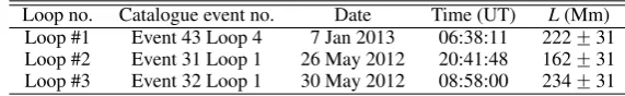
Table 1.Selected SDO/AIA observations of standing kink modes used in the paper.
Loop no. Catalogue event no. Date Time (UT) L(Mm) Loop #1 Event 43 Loop 4 7 Jan 2013 06:38:11 222˘31 Loop #2 Event 31 Loop 1 26 May 2012 20:41:48 162˘31 Loop #3 Event 32 Loop 1 30 May 2012 08:58:00 234˘31
pixel and temporal cadence of 12 seconds. A series of 100 such slits were created for each loop at different points along the axis and the slit which maximised the clarity of the TD map and the apparent amplitude of the oscillation was then chosen for further analysis. The chosen events are listed in Table1 which shows the designation (loop no.) by which they will be referred to in this paper, the designation used inGoddard et al.(2016), the date and time of the event, and the estimated loop lengthLwhich will be used in Sect.3. Figure1shows SDO images of the selected events.
3. Seismological inversion for damping due to mode coupling
Pascoe et al. (2013) produced a general spatial damping pro-file which describes the damping envelope of propagating kink waves for all times. It is based on the full analytical solution derived by Hood et al.(2013) and consists of two approxima-tions combined together; a Gaussian profile for early times with damping length Lg, and an exponential profile for later times with damping lengthLd;
Apzq “
$
&
%
A0exp
´
´2zL22 g ¯
zďh Ahexp
´
´z´Ldh
¯
ząh (1)
where Ah “ Apz“hqand the height at which the switch in profiles occurs is determined by the damping lengths
h“L2g{Ld. (2)
In this paper we consider standing kink modes which are instead characterised by considering a fixed point in space and measur-ing the variation of the oscillation amplitude in time. We can employ the same general damping profile using the change of variablet “ z{Ck, which corresponds to the long wavelength
limit for which the kink mode phase speed is the kink speed Ck. For a standing mode with wavelengthλin a coronal loop of lengthLwe have
Ck“λ{P (3)
withλ“2Lfor the global or fundamental standing mode. The damping time and length scales are related to the coronal loop transverse density profile by
τg P “
Lg
λ “
2
πκϵ1{2 (4)
τd P “
Ld
λ “
4
π2ϵκ (5)
whereϵ “ l{Ris the normalised inhomogeneous layer width andκ “ pρ0 ´ρeq{pρ0 `ρeqis a ratio of the internal density ρ0 and the external density ρe. The constant of proportional-ity depends upon the chosen densproportional-ity profile in the inhomoge-neous layer. Here we use a profile that varies linearly fromρ0 atrď pR´l{2qtoρeatrą pR`l{2q, this being the only pro-file for which the full analytical solution is currently known. The constant of proportionality is known for the exponential compo-nent of the general damping profile for the case of other profiles (e.g. see discussions byGoossens et al. 2002;Roberts 2008).
The general damping profile for standing kink waves is thus given by
Aptq “
$
&
%
A0exp
´
´2tτ22 g ¯
tďts Asexp
´
´t´ts τd
¯
tąts
(6)
whereAs“Apt“tsqand the switch in profiles is at
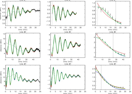
[image:4.595.157.443.301.345.2]Fig. 2.Kink oscillations fitted with a general damping profile. The left panels show the locations of the loop axis as a function of time for the three loops we consider. The background trends are shown by the dashed lines, and the detrended signals are shown in the middle panels. The right panels show the absolute values of the detrended extrema with the damping envelopes. The best fit curves correspond to exponential (red), Gaussian (blue), and general damping (green) profiles. The vertical dotted and dashed lines denote the start time of the oscillation and the switch timets, respectively.
Table 2.Fitted parameters for kink oscillations as defined by Eqs. (6) and (9).
Loop no. A0(Mm) ϕ(rad) P(min) τg(min) τd(min) ts(min) c0(Mm) c1(Mm/min) c2(Mm/min2)
Loop #1 0.98˘0.02 0.07˘0.03 4.73˘0.01 10.80˘0.27 6.35˘1.52 18.35˘4.29 3.89 0.083 ´0.0022 Loop #2 ´3.95˘0.02 ´0.18˘0.01 7.65˘0.01 17.87˘0.15 12.63˘0.83 25.29˘1.62 9.14 ´0.266 0.0043 Loop #3 ´2.37˘0.03 ´0.03˘0.01 4.17˘0.00 7.35˘0.24 8.81˘0.89 6.14˘0.48 10.53 ´0.045 ´0.0003
Table 3.Seismologically determined loop parameters.
Loop no. ρ0{ρe ϵ R(Mm) l(Mm) Ck(Mm/s) CA0(Mm/s) CAe(Mm/s) B0(G) Loop #1 1.69˘0.56 1.17˘0.39 1.54˘0.13 1.80˘0.62 1.56˘0.22 1.40˘0.30 1.82˘0.49 9.38˘2.56 Loop #2 1.87˘0.17 0.81˘0.07 2.59˘0.64 2.10˘0.56 0.71˘0.14 0.62˘0.12 0.85˘0.17 4.37˘0.88 Loop #3 5.25˘0.58 0.28˘0.04 3.34˘0.34 0.94˘0.15 1.87˘0.25 1.44˘0.21 3.30˘0.51 17.06˘2.63
Nc“ ts P “
h
λ “
1
κ “
ρ0`ρe
ρ0´ρe
“ ρ0{ρe`1 ρ0{ρe´1
(8)
whereNcis the number of cycles of the oscillation after which the switch occurs. We therefore expect loops with larger density contrasts to transition from the Gaussian profile to the exponen-tial one sooner than loops with smaller density contrasts. This forms the basis of the seismological method of determining κ
for an observed oscillation. The value of ϵ can then be calcu-lated from the relation in Eq. (4) or (5).
[image:5.595.63.552.594.639.2]Pascoeet al.: Kink mode seismology
damped sinusoid of the form
Aptqsinpωt´ϕq. (9)
The parametersA0,P “2π{ω,ϕ,τg,τd, andtsare determined by a Levenberg-Marquardt least-squares fit, with data points weighted according to their errors. The fitted values are given in Table2.
The background trend determined by spline interpolation al-lows the damped sinusoidal component of the oscillation to be identified as clearly as possible for accurate fitting of the damp-ing profile. However, such trends cannot conveniently be numer-ically quantified and so in Table2we also give the parameters for a second order polynomial trend of the formc0`c1t`c2t2 which approximates the interpolated trend. This polynomial ap-proximation is used in Sect.4to produce the forward modelled TD maps (see Fig.6).
Figure3shows the seismological inversions forρ0{ρeandϵ based on the kink mode damping profiles in Fig. 2. Using the exponential damping timeτdalone produces a curve of possible values as discussed byArregui et al.(2007) andGoossens et al.
(2008), whereas using the general damping profile given by Eq. (6) produces unique seismological inversions (red sym-bols), i.e. single pairs of values forρ0{ρeandϵ, within a
nar-row range (error bars) associated with observational uncer-tainty, fitting accuracy, and the propagation of these errors through the calculations discussed below.
Our least-squares fit of the general damping profile returns the parameters (and error estimates)P˘δP,τg˘δτg, andts˘δts. The seismological inversion is then calculated as
τd “ τ2g{ts
δτd “ |τd|
b
4`
δτg{τg˘2` pδts{tsq 2
κ “ P{ts
δκ “ |κ|
b
pδP{Pq2` pδts{tsq 2
ρ0{ρe “ p1`κq { p1´κq δpρ0{ρeq “ |ρ0{ρe|
b
2pδκ{κq2
ϵ “ 4P{`τdπ2κ˘
δϵ “ |ϵ|
b
pδP{Pq2` pδτd{τdq2` pδκ{κq2. (10)
We point out that our fitting routine considers all three of
τg,τd, andtssimultaneously as given by Eq. (6), though only
two of them are fitted independently and the third (hereτd)
given by Eq. (7).The values ofρ0{ρeandϵ are also given in Table3. Additional loop parameters in Table3 are determined as described below and in Sect.4.
The observational estimate for the loop length L ˘ δL (Table1) is used to calculate the kink speed using Eq. (3). In this paper we use the values given inGoddard et al.(2016).We can then determine the Alfv´en speeds inside (CA0) and out-side (CAe) the coronal loop, subject to the approximation that the magnetic field strength is constantB0 “Be, consistent with the lowβstate of plasma in coronal active regions. This is possi-ble since we have determined the density contrast independently, by the seismological inversion of the damping profile. However, the seismological determination of magnetic field strength still requires the absolute value of the density to be known by some additional measurement or method. The calculations performed
and associated errors are
Ck “ 2L{P δCk “ |Ck|
b
pδL{Lq2` pδP{Pq2
CA0 “ Ck{
b
2{ p1`ρe{ρ0q
δCA0 “ |CA0|
b
pδL{Lq2`2pδP{Pq2` pδts{tsq 2
CAe “ CA0
b
ρ0{ρe
δCAe “ |CAe|
b
pδL{Lq2`3pδP{Pq2`2pδts{tsq 2
B0 “ CA0
a
µ0µ¯mpn0
δB0 “ |B0|
b
pδL{Lq2`3pδP{Pq2`2pδts{tsq2, (11)
whereµ0“4πˆ10´7H/m, ¯µ“1.27,m
p“1.6726ˆ10´27kg, n0 “ neρ0{ρe, and here we assume a typical value of ne “ 1015 m´3(with no associated error). This estimate forn
eis the only parameter not determined from the observational data by the seismological method described in this paper. We bring to the reader’s attention that the errors in the Alfv´en speeds andB0 can be written in terms of the error in the time of the switch be-tween profilests (as well as the usualδL andδPterms), since this time determines the density contrast ratio which the kink speed depends on. An additional term of 0.25pδn0{n0q
2 is also required forδB0in the case of a measuredn0with known error δn0.
4. Forward modelling of time distance maps
In Sect.3we considered the time-dependence of the oscillating loop and performed a seismological inversion to determine coro-nal loop parameters. In this section we use this information and the intensity profiles perpendicular to the loop axis to determine further loop parameters. In particular, we use the seismologi-cally determined density contrast ratio and normalised inhomo-geneous layer widthϵ “ l{Rto then calculate the inhomoge-neous layer widthland loop radiusRseparately. This allows the transverse loop density profile to be determined, and by combin-ing this information with the time-dependence from Sect.3we will create forward modelled TD maps.
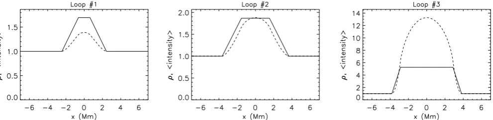
Figure4shows examples for each loop of Gaussian (dashed green) and forward modelled (solid blue) fits to the observed transverse intensity profile. Each of these fits represents a single instance in time during the oscillation (this estimation assumes that the loops do not perform unresolved, short-period oscilla-tions during the SDO/AIA integration time). For each loop, ap-proximately 100 such fits are used to calculate the mean valueR (and standard deviationδR) given in Table3. The corresponding density profiles (normalised to the external density) are given by the solid lines in Fig.5.
Fig. 3.Seismological inversions for the density contrast ratio and normalised layer width based on the kink mode damping profile. Using the exponential damping timeτdalone produces a curve of possible values (error bars denoted by dashed lines). Using the general damping profile given by Eq. (6)determinesϵandρ0{ρesimultaneously(red symbols with error bars).
Fig. 4.Examples of fitting observational transverse intensity profiles with Gaussian (dashed green) and forward modelled (solid blue) fits. The vertical lines are the corresponding locations of the loop centre for each fitted profile.
Fig. 5.Profiles for the seismologically determined transverse density (solid lines) and the corresponding averaged LOS intensity (dashed lines) for a cylindrical loop.
is smoother, due to the cylindrical symmetry. For example, the density is constant in the core region near the centre of the loop whereas the corresponding intensity varies continuously since the thickness of the core region (and the entire loop) along the LOS is greatest at the centre of the loop. Similarly, near the out-side edge of the inhomogeneous layer both the average loop den-sity and the thickness of the loop along the LOS are decreasing with increasing distance from the loop centre.
Both the Gaussian and forward modelled intensity profiles in Fig.4also include a background term in the form of a second order polynomial (in position). The vertical lines are the cor-responding locations of the loop centre for each fitted profile. The Gaussian and forward modelled profiles are both symmetric functions (although the background term may be asymmetric) and so give the same value for the location of the loop axis de-fined as the local maximum. The purpose of using the forward modelled profile is that the fit returns a value of loop radiusR which has the same definition as the density profile used in the
mode coupling model in Sect.3(and withϵconstrained to the seismologically determined value). On the other hand, fitting a Gaussian profile to the intensity returns a width or standard de-viationσ. We expect thatσ „Rbut with some unknown con-stant of proportionality of order unity (indeed comparing our fit-ting for Rfrom the forward modelled profile withσ from the Gaussian fitting gives usσ{R«0.6´0.7 for our three loops). Additionally, there is no expression to determinelfromσ, i.e.σ is freely fitted parameter for the Gaussian fit, whereas for the for-ward modelled profileRis free butϵ “l{Ris known and fixed for the particular loop. From our fitting of the forward modelled density profiles to the observed intensity profiles we haveR˘δR. The seismologically determinedϵfrom Eq. (10) then gives
l “ ϵR δl “ |l|
b
[image:7.595.57.553.393.514.2]Pascoeet al.: Kink mode seismology
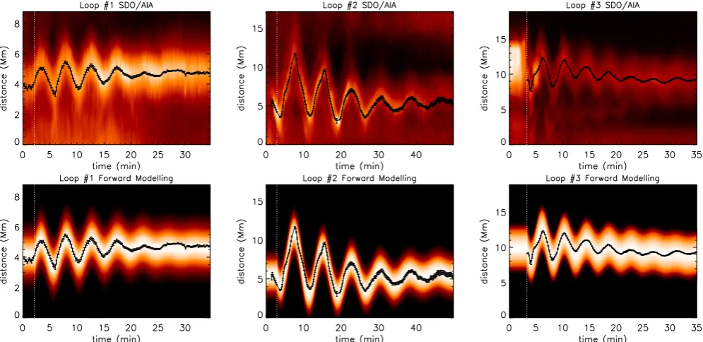
Fig. 6.Comparison of observational TD maps (top) with those produced by forward modelling (bottom) using the parameters given in Tables2and3. The vertical dashed lines denote the start time of the oscillation. The symbols are the fitted locations of the loop centre for the observational data (see also Fig.2).
Figure6 shows the observational (top panels) and forward modelled (bottom panels) TD maps. The forward modelled maps use the parameters given in Tables2and3(including the polyno-mial trend rather than the spline trend used in Sect.3). The verti-cal dashed lines denote the start time of the oscillation. For con-venience, the loop position is taken to be fixed before this time in the forward modelled TD maps. The symbols are the fitted loca-tions of the loop centre for the observational data, as also shown in the left panels of Fig.2. Since the forward modelling is based on the measured oscillation of a single loop, it only reproduces the intensity contribution from that loop, i.e. other structures or variations in the background intensity are not reproduced. The forward modelling also only considers the density dependence, and the density profile itself is taken to remain fixed during the oscillation. Variations in intensity due to variations in the den-sity or temperature are therefore not considered. In context of these features and limitations, the forward modelled TD maps demonstrate good agreement with the observational maps.
Next we briefly discuss two examples of further analysis of the observed coronal loops which are made possible by the in-formation about the transverse loop structure revealed by the method in this paper.
4.1. Dispersion diagrams
Information about the Alfv´en speed profile allows us to cal-culate the dispersion diagrams for the particular coronal loop. In Eq. (11) the kink speed is determined by the observed loop length and period of oscillation, which is based on the assump-tion that the oscillaassump-tion phase speed Vp is the kink speed Ck. Using the seismologically determined loop density contrast ra-tio (and the assumpra-tion of a constant magnetic field) then gives the internal and external Alfv´en speeds, which we use to calcu-late the dispersion diagrams. Using the loop radius found above then allows us to check the consistency of the long wavelength approximation used in our seismological method.
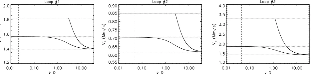
Figure7shows the dispersion diagrams for the three loops, i.e. the phase speed as a function of the wavenumberk“2π{λ normalised by the loop minor radiusR. The upper, middle, and lower dotted lines representCAe,Ck, andCA0, respectively. A logarithmic scale is used to emphasise the behaviour in the long wavelength limitkR!1 for which the kink mode phase speed tends to Ck. The other branch in each of the dispersion dia-grams corresponds to the sausage mode for which the phase speed tends toCAe at some finite cut-offwavenumberkcR „1, beyond which the sausage mode experiences leakage from the loop. The dashed lines correspond to the value for the global standing modekR“πR{Land so in each case demonstrate that the long wavelength approximation Vp « Ck is consistent. In each case we are also well within the leaky regime for sausage modes. Sausage modes do not experience mode coupling but due to leakage we would expect any excited sausage modes to have a low signal quality for loops with a small density contrast ratio (e.g.Cally 1986;Pascoe et al. 2007b;Vasheghani Farahani et al. 2014). On the other hand Nakariakov et al. (2012) show that the period depends on the transverse density profile in the long wavelength limit which may provide additional seismological diagnostics.
The dispersion diagrams in Fig. 7 are calculated us-ing the analytical solution for a magnetic cylinder given by
im-Fig. 7.Dispersion diagrams for the analysed loops showing the phase speedVpof the kink and sausage modes as a function of the normalised wavenumberkR. The upper, middle, and lower dotted lines representCAe,Ck, andCA0, respectively. A logarithmic scale is used to emphasise the behaviour in the long wavelength limitkR !1. The dashed lines correspond to the value for the global standing modekR“πR{L.
portant forϵ ≳ 1, and so might be relevant for our loops 1 and 2.Yu et al.(2015) also show that the choice of density pro-file in the inhomogeneous layer has a small effect on the period of oscillation for standing kink modes in magnetic slabs. The diagrams also assume plasma β “ 0, and we do not consider fluting modes or higher transverse harmonics of the sausage and kink modes.
4.2. Phase mixing and heating
The transfer of energy from collective transverse loop motions (kink waves) to localised azimuthal motions (Alfv´en waves) by mode coupling is an ideal process. All the energy of the ini-tial kink oscillation is eventually converted to Alfv´en waves. In a uniform medium, Alfv´en waves are very weakly dissipated. However, the mode coupling process we consider requires the Alfv´en waves are generated in a non-uniform medium, i.e. the inhomogeneous layer of the coronal loop. The continuous varia-tion of the the local Alfv´en speed with posivaria-tion means the Alfv´en waves will experience phase mixing which generates large trans-verse gradients in the waves (e.g.Heyvaerts & Priest 1983;Cally 1991; Hood et al. 2005; Soler & Terradas 2015). Equivalently, we can consider the characteristic spatial scale of the perturba-tions to be the phase mixing lengthLph, which continuously de-creases in time. The seismological method presented in this pa-per gives information about the Alfv´en speed profile transverse to the loop (see Fig.5) which can be used to study the dissipa-tion of the wave energy and consequent heating of the plasma. Here we present some simple estimates based on the assumption that the efficiency of the Alfv´en wave dissipation mechanism is inversely proportional to the characteristic spatial scale of the wave, which is itself determined by phase mixing.
Phase mixing is a common phenomenon and has been stud-ied in detail in several contexts. For Alfv´en waves in the Earth’s magnetospshere Mann et al.(1995) calculated the time depen-dence of the phase mixing length as
Lph“ 2π ω1
At
(13)
whereω1
A « k||v1A and for our model with a linear profile in the inhomogeneous layerv1
A“ pCAe´CA0q {l. This approxima-tion was also found to accurately describe simulaapproxima-tions of Alfv´en waves generated by mode coupling of kink waves propagating along coronal loops byPascoe et al.(2010).
Mann & Wright (1995) estimated the lifetime of poloidal Alfv´en waves in the Earth’s magnetosphere as τA “ ka{ω1A
whereka is the azimuthal wavenumber. For kink modeska “ 1{R, and the Alfv´en waves generated by mode coupling retain this (m“1) symmetry. We can therefore rewriteτAin terms of the parameters used in this paper as
τA“ ϵL
πpCAe´CA0q.
(14)
The estimatesof this phase mixing timescalefor loops 1–3 are 197, 185, and 11 seconds, respectively. Evidently, thetimescale
is strongly dependent on the loop density contrast ratio which determines the change in Alfv´en speed. While the Alfv´en waves themselves cannot be resolved by modern instruments,these dif-ferent phase mixing timescales may contribute to different heating rates for the loops. It may be possibleto detect signa-tures of such variations in heating rates for different loops.The role of mode coupling in plasma heating has recently been studied byOkamoto et al.(2015) andAntolin et al.(2015) for transverse oscillations of prominences, in which the Kelvin-Helmholtz instability also generates small spatial scales in the inhomogeneous layer to allow efficient dissipation of the wave energy.
5. Discussion and conclusions
The full seismological method used in this paper is summarised below, with a note of the particular assumptions or approxima-tions employed.
1. Produce TD map for observational data such as SDO/AIA. The loop length is also estimated separately to calculate the kink mode wavelength and hence the kink speedCk using Eq. (3).
2. Use observational TD map to determine time series for the loop position, e.g. Gaussian fit of the transverse intensity to determine the position of the loop centre.
3. Fit detrended time series with damped sinusoidal oscilla-tion with the envelope being the general damping profile in Eq. (6). The density profile in the inhomogeneous layer is assumed to be linear (this being the only profile for which a full analytical solution is currently known).
4. Use fitted general damping profile parameters for seismolog-ical inversion to determine the loop density contrast ρ0{ρe with Eq. (8), and the inhomogeneous layer width ϵ with Eq. (4) or (5) (see also Eq. (10)).
[image:9.595.57.554.58.176.2]ap-Pascoeet al.: Kink mode seismology
proximation of a constant magnetic fieldB0 “ Be. The ex-ternal Alfv´en speedCAecan be determined similarly, and if the plasma densityρ0orρeis known or can be estimated the magnetic field strengthB0can also be calculated.
6. Calculate the forward modelled intensity for the loop density profile using the calculated values ofρ0{ρe andϵ. Here we use the approximation that the temperature is constant and so the intensity is proportional toρ2integrated along the LOS. The loop is also assumed to be cylindrical. Comparison of this model intensity profile to the observational intensity pro-file determinesRby least-squares fitting, and hencelfrom Eq. (12).
7. Having obtained the Alfv´en speed profile for the coronal loop additional physical calculations can then be performed. For example, the dispersion diagrams (Sect.4.1) or the phase mixing rate (Sect.4.2).
The most important and novel component of this methodin comparison with previous observational studiesis the use of the general damping profile given by Eq. (6) to describe the de-cay of the kink oscillation due to mode coupling. Fitting this profile determines two damping timescales,τg for the Gaussian regime andτd for the exponential regime, and so provides us with an additional independent observable,making the prob-lem well-posed and allowing a seismological inversion to be performed which provides specific values for the density contrast ratio and normalised inhomogeneous layer width (within errors). Fitting only the Gaussian or exponential com-ponent of the profile gives a single timescale and so the seis-mological inversion is a curve in parameter space, such as those shown in Fig.3.
This method not only allows the loop density contrast ratio to be estimated, but also does so in a method which is inde-pendent of intensity or spectral measurements. The method re-quires that the effects of LOS integration in the corona permit the loop to be accurately tracked during its oscillation. However, if this is satisfied the subsequent estimates ofρ0{ρe andϵ are not affected by LOS integration effects (e.g.Cooper et al. 2003;
De Moortel & Pascoe 2012;Viall & Klimchuk 2013).
The seismological determination of the magnetic field strength B0 of coronal loops by observations of standing kink oscillations depends on four parameters; L, P, ρ0{ρe, and ρ0. The loop length and period of oscillation are determined di-rectly from observational data, and the density contrast ratio is revealed by our method. However, some other method or ob-servation is required forρ0 and so for this reason the magnetic field strengths given in Table3 remain dependent upon an as-sumed parameter. In any case the method we present is an im-proved technique for the description of the damping profile of the kink mode, and can be a powerful component of a larger seismological strategy which includes, for example, simulta-neous observation of additional harmonics (e.g. Andries et al. 2005; Srivastava et al. 2013) or wave modes (e.g.Zhang et al. 2015), spatial seismology using time series from different lo-cations (e.g.Verth et al. 2007;Pascoe et al. 2009b), temperature data from multiple bandpasses (e.g.Cheung et al. 2015), or in-formation about the magnetic field from extrapolations (e.g. Verwichte et al. 2013) or modelling (e.g.Chen & Peter 2015), in addition to any improvements to the theoretical modelling of the relevant physical processes.
Acknowledgements. This work is supported by the Marie Curie
PIRSES-GA-2011-295272 RadioSun project, the European Research Council under the
SeismoSunResearch Project No. 321141 (DJP, CRG, SA, VMN) and the STFC
consolidated grant ST/L000733/1 (GN, VMN). The data is used courtesy of the SDO/AIA team.
References
Andries, J., Arregui, I., & Goossens, M. 2005, ApJ, 624, L57
Andries, J., van Doorsselaere, T., Roberts, B., et al. 2009, Space Sci. Rev., 149, 3
Anfinogentov, S., Nistic`o, G., & Nakariakov, V. M. 2013, A&A, 560, A107 Anfinogentov, S. A., Nakariakov, V. M., & Nistic`o, G. 2015, A&A, 583, A136 Antolin, P., Okamoto, T. J., De Pontieu, B., et al. 2015, ApJ, 809, 72
Arregui, I. 2015, Philosophical Transactions of the Royal Society of London Series A, 373, 20140261
Arregui, I., Andries, J., Van Doorsselaere, T., Goossens, M., & Poedts, S. 2007, A&A, 463, 333
Arregui, I. & Asensio Ramos, A. 2014, A&A, 565, A78
Arregui, I., Asensio Ramos, A., & Pascoe, D. J. 2013, ApJ, 769, L34
Arregui, I., Van Doorsselaere, T., Andries, J., Goossens, M., & Kimpe, D. 2005, A&A, 441, 361
Aschwanden, M. J. 2009, Space Sci. Rev., 149, 31
Aschwanden, M. J., Fletcher, L., Schrijver, C. J., & Alexander, D. 1999, ApJ, 520, 880
Aschwanden, M. J. & Schrijver, C. J. 2011, ApJ, 736, 102 Cally, P. S. 1986, Sol. Phys., 103, 277
Cally, P. S. 1991, Journal of Plasma Physics, 45, 453 Chen, F. & Peter, H. 2015, A&A, 581, A137
Chen, L. & Hasegawa, A. 1974, Physics of Fluids, 17, 1399
Cheung, M. C. M., Boerner, P., Schrijver, C. J., et al. 2015, ApJ, 807, 143 Cooper, F. C., Nakariakov, V. M., & Tsiklauri, D. 2003, A&A, 397, 765 De Moortel, I. & Nakariakov, V. M. 2012, Royal Society of London
Philosophical Transactions Series A, 370, 3193 De Moortel, I. & Pascoe, D. J. 2009, ApJ, 699, L72 De Moortel, I. & Pascoe, D. J. 2012, ApJ, 746, 31
De Moortel, I., Pascoe, D. J., Wright, A. N., & Hood, A. W. 2016, Plasma Physics and Controlled Fusion, 58, 014001
Edwin, P. M. & Roberts, B. 1983, Sol. Phys., 88, 179
Goddard, C. R., Nistic`o, G., Nakariakov, V. M., & Zimovets, I. V. 2016, A&A, 585, A137
Goossens, M., Andries, J., & Aschwanden, M. J. 2002, A&A, 394, L39 Goossens, M., Arregui, I., Ballester, J. L., & Wang, T. J. 2008, A&A, 484, 851 Heyvaerts, J. & Priest, E. R. 1983, A&A, 117, 220
Hollweg, J. V. & Yang, G. 1988, J. Geophys. Res., 93, 5423
Hood, A. W., Brooks, S. J., & Wright, A. N. 2005, Proceedings of the Royal Society of London Series A, 461, 237
Hood, A. W., Ruderman, M., Pascoe, D. J., et al. 2013, A&A, 551, A39 Ionson, J. A. 1978, ApJ, 226, 650
Mann, I. R. & Wright, A. N. 1995, J. Geophys. Res., 100, 23677
Mann, I. R., Wright, A. N., & Cally, P. S. 1995, J. Geophys. Res., 100, 19441 McLaughlin, J. A. & Ofman, L. 2008, ApJ, 682, 1338
Nakariakov, V. M., Hornsey, C., & Melnikov, V. F. 2012, ApJ, 761, 134 Nakariakov, V. M. & Ofman, L. 2001, A&A, 372, L53
Nakariakov, V. M., Ofman, L., Deluca, E. E., Roberts, B., & Davila, J. M. 1999, Science, 285, 862
Nistic`o, G., Nakariakov, V. M., & Verwichte, E. 2013, A&A, 552, A57 Ofman, L. 2010, Living Reviews in Solar Physics, 7
Okamoto, T. J., Antolin, P., De Pontieu, B., et al. 2015, ApJ, 809, 71
Parnell, C. E. & De Moortel, I. 2012, Royal Society of London Philosophical Transactions Series A, 370, 3217
Pascoe, D. J. 2014, Research in Astronomy and Astrophysics, 14, 805 Pascoe, D. J. & De Moortel, I. 2014, ApJ, 784, 101
Pascoe, D. J., de Moortel, I., & McLaughlin, J. A. 2009a, A&A, 505, 319 Pascoe, D. J., Goddard, C. R., Nistic`o, G., Anfinogentov, S., & Nakariakov,
V. M. 2016, A&A, 585, L6
Pascoe, D. J., Hood, A. W., de Moortel, I., & Wright, A. N. 2012, A&A, 539, A37
Pascoe, D. J., Hood, A. W., De Moortel, I., & Wright, A. N. 2013, A&A, 551, A40
Pascoe, D. J., Nakariakov, V. M., & Arber, T. D. 2007a, Sol. Phys., 246, 165 Pascoe, D. J., Nakariakov, V. M., & Arber, T. D. 2007b, A&A, 461, 1149 Pascoe, D. J., Nakariakov, V. M., Arber, T. D., & Murawski, K. 2009b, A&A,
494, 1119
Pascoe, D. J., Wright, A. N., & De Moortel, I. 2010, ApJ, 711, 990 Pascoe, D. J., Wright, A. N., & De Moortel, I. 2011, ApJ, 731, 73
Pascoe, D. J., Wright, A. N., De Moortel, I., & Hood, A. W. 2015, A&A, 578, A99
Roberts, B. 2008, in IAU Symposium, Vol. 247, IAU Symposium, ed. R. Erd´elyi & C. A. Mendoza-Briceno, 3–19
Soler, R. & Terradas, J. 2015, ApJ, 803, 43
Srivastava, A. K., Dwivedi, B. N., & Kumar, M. 2013, Ap&SS, 345, 25 Stepanov, A. V., Zaitsev, V. V., & Nakariakov, V. M. 2012, Stellar Coronal
Seismology as a Diagnostic Tool for Flare Plasma Terradas, J., Arregui, I., Oliver, R., et al. 2008, ApJ, 679, 1611 Terradas, J., Goossens, M., & Verth, G. 2010, A&A, 524, A23 Tomczyk, S. & McIntosh, S. W. 2009, ApJ, 697, 1384
Tomczyk, S., McIntosh, S. W., Keil, S. L., et al. 2007, Science, 317, 1192 Van Doorsselaere, T., Andries, J., Poedts, S., & Goossens, M. 2004, ApJ, 606,
1223
van Doorsselaere, T., Nakariakov, V. M., Verwichte, E., & Young, P. R. 2008, in European Solar Physics Meeting, Vol. 12, European Solar Physics Meeting, ed. H. Peter, 2.81
Van Doorsselaere, T., Nakariakov, V. M., Young, P. R., & Verwichte, E. 2008, A&A, 487, L17
Vasheghani Farahani, S., Hornsey, C., Van Doorsselaere, T., & Goossens, M. 2014, ApJ, 781, 92
Verth, G., Terradas, J., & Goossens, M. 2010, ApJ, 718, L102
Verth, G., Van Doorsselaere, T., Erd´elyi, R., & Goossens, M. 2007, A&A, 475, 341
Verwichte, E., Van Doorsselaere, T., Foullon, C., & White, R. S. 2013, ApJ, 767, 16
Viall, N. M. & Klimchuk, J. A. 2013, ApJ, 771, 115 White, R. S. & Verwichte, E. 2012, A&A, 537, A49 Yu, H., Li, B., Chen, S.-X., & Guo, M.-Z. 2015, ApJ, 814, 60