Grobner Basis for Bivariate Normal with Missing Data Model Estimation Problem

(1)

ISSN: 1816-949X

Grobner Basis for Bivariate Normal with Missing Data Model Estimation Problem

1

_{Saad Abed Madhi and}

2

_{Saad Ali Sultan}

1

_{Department of Biomedical Engineering, Al-Mustaqbal University College, Babylon, Iraq}

2

_{Department of Mathematics, College of Education for Pure Science,}

University of Babylon, Babylon, Iraq

Abstract: The goal of this study is to study maximum likelihood estimates for a bivariate distribution with

missing data using an algebraic geometry tool, namely, Grobner basis techniques. In maximum likelihood estimation, the parameters of the model are estimated by maximizing the likelihood function which maps the parameters to the likelihood of observing the given data. By transforming this optimization problem into a polynomial optimization problem, it can be shown that the solutions of the likelihood equations can be computed using Grobner basis technique.

Key words:Bivariate normal distribution, Buchberger’s algorithm, Grobner bases, algebraic geometry,

maximum likelihood estimation, s-polynomial

INTRODUCTION

Originally, the method of Grobner bases was introduced by Buchberger (1965, 1970) for the algorithmic solution of some of the fundamental problems in commutative algebra (polynomial ideal theory, algebraic geometry). A Grobner basis technique was first introduced by Bruno Buchberger in his PhD dissertation research (1965) (Buchberger, 1970). They are named after Buchberger’s advisor, Wolfgang Groebner. Grobner basis technique is applied to solve systems of polynomial equations in several variables. In this study, we will use this technique to obtain the maximum likelihood estimation of the parameters in a bivariate normal distribution.

MATERIALS AND METHODS

Some definitions and theorems: We will assume that the

reader is familiar with the definitions of the following: ring and field.

Definition 2.1 (Cox et al., 1991): Let N denote the non-negative integers. Let α (α1, ..., αn) be a power vector

in Nn_{and let x}

1, ..., xn be any n variables. Then a

monomial xα in x1, ..., xn is defined as the product -_xα_{= x}

1

α1_{... x} n

αn_{. Moreover, the total degree of the}

monomial Xα is defined as |α| = α1 + ...+αn.

Definition 2.2 (Cox et al., 1991): Let k be any field and let f = 3α aα xα be a polynomial in k [x1, ..., xn]:

C We call aα the coefficient of the monomial xα

C If aα… 0, then we call aα xα term of f

The total degree of f denoted deg (f) is the maximum |α| such that the coefficient is a_α nonzero.

Definition 2.3 (Cox et al., 1991): Given a field k and a

positive integer n, we define the n-dimensional affine space over k to be the set kn_{= {(a}

1, ..., an): a1, ..., an k}. Definition 2.4 (Pistone et al., 2000): Let be a subset of ks_.

The set of polynomials defined by:

 









1 s 1 s

1 s

f k[x ,..., x ] : f a ,...,a Ideal S

0for all a ,...,a S

  

 

  



 

 

Is an ideal called ideal of S. The variety generated by a polynomial ideal I f k [x1, ..., xs] is:

 









s

1 s

a , ...,a K : Variety I =

f a , ...,a =0for allf I

  

 

 



 

 

A subset of Ks_{which is a variety of a polynomial}

ideal in k [x1, ..., xs] is called a variety.

Definition 2.5 (Cox et al., 1991): A subset I0k [x1, ..., xn]

is an ideal if it satisfies: C 00I

C If f, g 0I then f+g 0I

C If f 0I and h 0k[x1 ,..., xn] then h f 0I

Definition 2.6 (Cox et al., 2005): Let f₁, ..., f_s be polynomials in k [x₁ ,..., x_n]. We let <f₁, ..., f_s> denote the collection < f1, ..., fs> =









is an

s

i i 1 s 1 n

i 1h f :h , ..., h k x , ..., x



ideal.

(2)

Definition 2.7 (Adams and Loustaunau, 1994): A greatest common divisor of polynomials f, g0k [x] is a polynomial h such that:

C h divides f and g

C If p 0k [x] divides f and g then p divides h C LC (h) = 1 (that is h is monic)

Definition 2.8 (Cox et al., 1991): Let α and β in Nn_.

C Lexicographic order: α>_lex β if and only if the left-most nonzero entry in α-β is positive

C Graded lex order: α>grlexβ if and only if |α|>|β| or (|α|

= |β| and α >_lexβ)

C Graded reverse lex order (tdeg): α>grevlexβ if and only

if |α|>|β| or (|α| = |β| and the right-most nonzero entry in α-β is negative)

Definition 2.9 (Cox et al., 1991): Assume an arbitrary

admissible ordering >is fixed. Given a nonzero polynomial f 0k [x1, ..., xn], we define:

C The multidegree of f as: multideg (f) = max (α _Nn_:

αa… 0)

C The leading monomial of f as: LM (f) = xmultideg (f)

C The leading coefficient of f as: LC = (f) = α_{multideg (f)} C The leading term of f as: LT (f) = LCL (f). LM (f)

Theorem2.10:( Division Algorithm) (Cox et al., 1991):

Fix a monomial order >on and let F = (f1, ..., fs) be an

n 0

 

ordered s-tuple of polynomials in k [x₁, ..., x_n]. Then every f 0k (x1, ..., xn) can he written as fa f +...+a f +r1 1 s s where

ai, rk [x1, ..., xs] and either r = 0 or r is a linear

combination with coefficients in k of monomials, none of which is divisible by any LT (f1), ..., LT (fs). We will call

r a remainder of f on division by F.

Definition 2.11 (Pistone et al., 2000): Let I d k [x1, ..., xn]

be an ideal other than{0}:

C We denote by LT (I) the set of leading terms of elements of I . Thus, LT (I) = {cxα: there exists f 0 I with LT (f) = cxα}

C We denote by +LT(I), the ideal generated by the elements LT (I)

Proposition 2.12 (Pistone et al., 2000): Let I d k [x1, ...,

x_n] be an ideal:

C +LT (I), is a monomial ideal

C There are g₁, ..., g_s 0I such that +LT (I), = +LT (g1), ... , LT (gs),

Theorem 2.13: (Hilbert basis theorem) (Cox et al., 1991): Every ideal I d k [x1, ..., xn] has a finite

generating set. That is i = +g1, ..., gs, for some

g₁, ..., g_s0I.

Grobner basis: In this study we define the fundamental

object of this study, namely, Grobner basis.

Definition 3.1 (Cox et al., 1991): Fix a monomial order.

A finite subset G = {g₁, ..., g_s} of an ideal I is said to be a Groebner basis (or standard basis) if +LT (g1), ..., +LT

(gs), = +LT (I),. Equivalently, a set {g1, ... ,gs} d I is a

Groebner basis of I if and only if the leading term of any element of I is divisible by one of the LT (gi).

Corollary 3.2 (Adams and Loustaunau, 1994):

Every non-zero ideal I 0 k [x1, ..., xn] has a Groebner

basis.

Theorem 3.3 (Pistone et al., 2000): Let I be a non-zero

ideal of k [x1, ..., xn]. The following statements

are equivalent for a set of non-zero polynomials G = {g1, ..., gs} d I:

C G = {g1, ..., gs} is a Groebner basis for I

C f 0I if and only if G where means the

f 0

 _ G

f



remainder on division of f by the ordered s-tuple G C f 0I if and only if f



si 1h gi i with LT (f) = max (LT

(hi), LT (gi)) C LT (G) = LT (I)

S-polynomials and Buchberger’s algorithm: Before

describing the Buchberger algorithm we define S-polynomials (S). In particular S-S-polynomials are used to test whether a set of polynomials is a Groebner basis.

Definition 4.1 (Cox et al., 1991): Let f and g be two

polynomials in R. The S-polynomial of f and g is the following combination:

 

L

_{ }

L

_{ }

S f ,g .f - .g

LT f LT g 

where, L is the least common multiple. .

 





LLCM LT f , LT g

Theorem 4.2 (Cox et al., 1991): Let I be a polynomial

ideal. Then a basis G = {g1, ..., gs} is a Groebner basis for

I if and only if for all pairs i … j the remainder on division of S (gi, gj) by G is zero.

Theorem 4.3: (Buchberger’s algorithm) (Cox et al., 1991): Let I = +f1, ..., fs … {0} be a polynomial ideal. Then

a Groebner basis for I can be constructed in a finite number of steps by the following algorithm.

(3)

Output: A Groebner basis G = (g1, ..., gt) for I with F d

G G: = F

Repeat:

G’: = G

FOR each pair {p, q}, p … q in G’ DO

 

G '

S : S p,q

If S … 0 then G:= G U {S} Until G = G’

Definition4.4 (Adams and Loustaunau 1994): A

Groebner basis G = {g1, ..., gs} is called minimal if for all

i, LC (gi) = 1and for all, i … j, LP (gi) does not divide LP

(gi).

Definition 4.5 (Adams and Loustaunau 1994): A

Groebner basis G = {g₁, ..., g_s} is called a reduced Groebner basis if for all I, LC (gi) = 1 and gi is reduced

with respect to G - {g_i}. That is for all, no non-zero term in gi is divisible by any LP (gj) for any i … j.

Definition 4.6 (Cox et al., 1991): A minimal Groebner

basis for a polynomial ideal I is a Groebner basis G for I such that:

C LC (p) = 1 for all p 0G

C For all p0 G LT (p) ó+LT (G-{p}),

RESULTS AND DISCUSSION

Computation: maximum likelihood estimation and Grobner basis

Maximum likelihood estimates for a bivariate

distribution with missing data: The Maximum

Likelihood Estimators (MLE) are obtained for the parameters of a bivariate normal distribution with equal variances when some of the observations are missing on one of the variables.

Maximum likelihood estimates: Let us consider the

incomplete bivariate sample:

1 n n +1 N

1 n

x , ..., x , x , ..., x

y , ..., y

From a bivariate normal distribution with mean vector (μ1, μ2) and a covariance matrix with common

variance σ2_{and correlation coefficient}_ρ_{. It may be noted}

that (x_i, y_i), i = 1, ..., n are paired observations. The likelihood function can be written as:

(1)









 





 









- N +n / 2 -n/2

2 2

1 2

N 2

i 1 i 1

2 2 2

2 N

i 2 i 1

i 1

L , , , 2

1-x - 1

-

-2 2

1-×exp

y - - x

-



      

 _ 

 

    

 

 _{ } _ 

 



The log-likelihood function is:

(2)





 





 









N 2

i 1 2 i 1

2

2 n

i 2 i 1

2 2 i 1

x -n

log L - N+n log - log 1- -

-2 2

1

y - - x -2

1-





  

   

 



Take the partial derivatives of log L with respect to μ1, μ2, σ2 and ρ equate them to zero and rearrange the

equations, we get:

(3)

N 2 N 2 n

i 1 i 1 i

i 1 i 1 i 1

n

2 2

2 i 1 i 1

x -N - x +N - y +

n + x -n 0

  



    

     



(4)

n n

i 2 i 1

i 1y -n - i 1x +n  0



(5)









i

N N

2 2 2 2

i 1 i

i 1 i 1

N N n

2 2 2 2 2 2 2

1 i 1 i 1 i 1 i 1 i 1 i

n ₂ n n

2 i 1 i 2 i 1 i i 2 i 1 i

n 2 n 2 2 n

1 i 1 i 1 2 i 1 i 1 i 1

2 2 1

- N+n + N+n + x -2 x +

N - x +2 x -N + y

-2 y +n -2 x y +2 x +

2 y -2n + x -2 x +

n 0

 

  

   

     

    

      

  



(6)

n n

2 2 3

i i 1 i 2

i 1 i 1

n n 2 n

i 1 2 i 2 i

i 1 i 1 i 1

n n n

2 2 2

2 i 1 i i 1 i 1 i 2 2 i 1 i

n n

2 2 2

1 2 i 1 i 1 i 1 i 1

n -n + x y - y

-x +n - y +2 y

-n + x y - y - x +

n - x +2 x -n 0

 

  

 

    

    

      

        



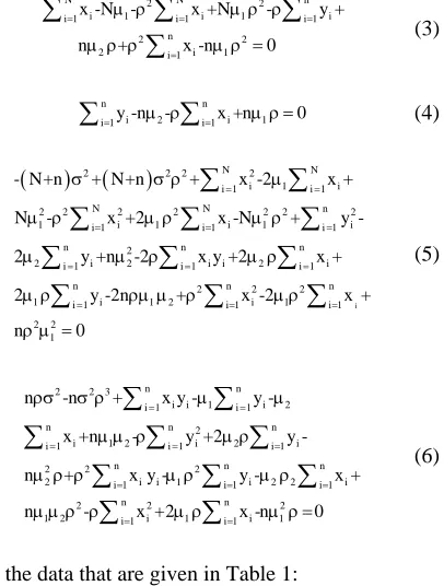
Using the data that are given in Table 1:

N n n

i i i

i 1 i 1 i 1

N 2 n 2 n 2 n

i i i i i

i 1 i 1 i 1 i 1

N 5, n 3, x 15, x 6, y 9,

x 55, x 14, y 29 and x y 19

  

   

    

   



[image:3.612.339.542.319.587.2]



Table 1: Data

i xi yi

2 i

x 2

i

y x yi i

1 3 3 9 4 9

2 1 2 1 16 2

3 2 4 4 9 8

4 5 - 25 -

-5 4 - 16 -

(4)

The Eq. 2-5 become:

(7)

2 2

1 1 2

15-5 -9 +2 -9 +3   0

(8)

2 1

3- -2 +   0

(9)

2 2 2 2 2 2 2 2

1 1 1 1

2

2 2 2 1 1 2

-8 +8 +84-30 +5 -41 +18 -2

-18 +3 -38 +112 +18 -6 0

         

         

(10)

2 2 3 2

1 2 1 2 2 2

2 2 2 2 2

1 2 1 2 1 1

3 -3 +19-9 -6 +3 -43 +18 -3 +

19 -9 -6 +3 +12 -3 0            

            

Now we will apply Grobner basis method to solve this system of polynomials, let:

(11)

2 2

1 1 1 2

f 15-5 -9 +2  -9 +3  

(12)

2 2 1

f  3- -2 +  

(13)

2 2 2 2 2 2

3 1 1 1

2 2 2

1 2 2 2 1 1 2

f -8 +8 +84-30 +5 -41 +18

-2 18 +3 -38 +12 +18 -6

        

          

(14)

2 2 3

4 1 2 1 2 2

2 2 2 2 2 2

2 1 2 1 2 1 1

f 3 -3 +19-9 -6 +3 -43 +18

-3 +19 -9 -6 +3 +12 -3

         

              

To solve these equations we consider the ideal F = +f1, f2, f3, f4, and choose the lexicographic order where

μ1>lexμ2>lexσ>lexρ. We will finding S-polynomial of f1 and

f₂. Since:

 

2

 

1 1 2 1

LT f   2 and LT f   

Then:

 







2 1



22

1 1 1

L LCM LT f , LT f

LCM 2 , 2

 

      



1 2



_{ }

1

_{ }

2

1 2

L L

S f ,f .f - .f LT f LT f 









2 2

1 1

1 2 2

1 2 1

2

2 1 1 2

15-15 -9 +2

-2 2

S f ,f

-2 9 +3

3- -2 + 15-5 -5 -15 +5      

   

 _{ } _ _ _{ }

  

 

         

And:





F ₂

1 2 1 2

S f ,f 15-15 -5 -15 +5   0

Therefore, we must add:

(15)

2

5 1 1 2

f 15-15  -5 -5 -15 +5  

To the generating set. The ideal becomes:

1 2 3 4 5

F = f ,f ,f ,f ,f

And:





F 1 2

S f ,f 0

Similarly:





2 2 2

1 3 1 2 1

2 2 2

1 2 2 2 1

S f ,f 3 +8 -8 -84+15 +

41 -9 +18 -3 +38 -12 -9                  





F

2 2 2 2

1 3

S f ,f = -12-8  +2 +8  +8 0

(16)

2 2 2 2

6

f -12-8  +2 +8  +8





F 1 2 3 4 5 6 1 2

F f ,f ,f ,f ,f ,f andS f ,f 0

Similarly:





2 2 3 2 2 2

1 4 1 2

2 2 2 2 2

1 1 2 1 2 1 1

3 2 2 2 2

1 1 2 1 1 2 1 2

2 2 2

1 2 1

S f ,f -45 +27 +9 -9 +

27 -38 +12 -6 +86 -24 +

6 -36 +18 +6 +12

-6 -38

                                      

And:





F ₂

1 4 2 1 2

2 3 3 2

1 2 1 2 1 2

S f ,f -237+353 -184 -135 +

60 +45 -15 +15 -15 0

   

       

(17)

2

7 2 1 2

2 3 3 2

1 2 1 2 1 2

f -237+353 -184 -135 +

60 +45 -15 +15 -15

   

      

To the generating set. The idealo becomes:





F 1 2 3 4 5 6 7 1 4

F f ,f , f , f ,f ,f ,f and S f ,f 0

Similarly:





 



2 2 2

1 5 2 2 2 1 2 2

F

3 2 2

2 1 1 1 1 1 5

S f ,f 75 -45 -45 -25 +15

-45 -30 +10 +10 +30 S f ,f 0          

          

And similarly:





2 2 2 2 2

1 6 1 2

2 3

1 1 1

S f ,f -60 +36 +12 -12 +

36 +12 -12 -8

              

(5)





F

1 6 1 2

S f ,f -6+2 +4 +2 0

(18)

8 1 2

f -6+2 +4 +2









F

1 2 3 4 5 6 7 8 1 6

F f ,f ,f ,f ,f ,f ,f ,f and S f ,f 0

Similarly:





2 2

1 7 1 2 1 2 1 2

2 2 3 2

2 1 1 2 2

2 2 2 2 2 5 3 2

1 2 1 2

S f -f -225 +15 +75

-45 +135 +474 -14 -706 +

368 +270 -90 +30 -30                  

        

And:





F

1 7 2

S f ,f -54-18 +18  0

(19)

9 2

f -54-18 +18 





F 1 2 3 4 5 6 7 8 9 1

F f ,f ,f ,f ,f ,f ,f ,f ,f and S f ,f 7 0

Similarly:





2 2 2 2 2 3

3 4 2 1 1 2 1

4 2 2 4 3 2 2 3

1 2 1

2 2 2 3 4 3 2 2

2 1 1 2 1 1

2 2 2 2 3 2 2 2

1 1 1 2 1

3 2 2 2 2 2 2 3

1 2 1 2 1 1

S f ,f -36 +90 -12 +24 +

24 +18 -24 +114 -18

-9 -86 +6 -6 -18 -252 +

38 +38 +123 +36 -54 +

6 -6 -9 -54 +54

                                

                      2

2

 

And:





F

2 2 2

3 4

65

S f ,f 11- -10 +18 +20 0 2

      

(20)

2 2 2

10

65

f 11- -10 +18 +20 2

     





F

1 2 3 4 5 6 7 8 9 10 3 4

F f , f , f , f , f , f , f , f , f , f and S f ,f 0

Similarly:





2 2 2 2 2

3 5 2 2 2 2 1 2

2 2 3

1 2 1 2 2 2 2 1 2

2 2 2 2 3 3 2 2

2 1 2 1 1 1 1

f , f 40 +420 +40 -205 +90

-150 +25 -90 +15 190 +90 +

60 -30 +30 -10 -10 -30

           

          

           

And:





F

3 2

3 5

40 20 10 S f ,f - -40 + 0

3 3 3

    

(21)

3 2

11

40 20 10 f - -40 +

3 3 4

   





F 1 2 3 4 5 6 7 8 9 10 11 3 5

Ff ,f ,f ,f ,f ,f ,f ,f ,f ,f ,f andS f ,f 0

Similarly:





4 2 2 2 2 2 2 2

3 10 1

2 2 2 2 2 2 2 2

1 1 2 2 1

2 2 2 2 2 2 2 2 2 3

2 1 1 1 1 1

f ,f -80 +840 +80 -410 +180

-300 +50 -180 +30 -380 +180 +

65

120 -60 +11 - -10 +6

2

        

            

               

And:





F ₂ ₃

3 10

405 27

S f ,f - + +135 -81 0 2 4

    

(22)

2 3

12

405 27

f - + 135 -81 2 4

   





F 1 2 3 4 5 6 7 8

3 10 9 10 11 12

f ,f ,f ,f ,f ,f ,f ,f ,

F andS f ,f 0

f ,f ,f ,f

 

Similarly, since, the reminders of the S-polynomials for all pairs polynomials f8, f9, f11 and f12 are zero,

therefore, the Groebner basis of F is:

8 9 11 12 1 2

3 2 2 3

2

G f ,f ,f ,f <-6+2 +4 +2 ,-54-18 +

40 20 10 405 27

18 , - -40 + ,- + +135 -81

3 3 3 2 4

     

       

So that, the reduced (minimum) Groebner basis of ideal F is:

2 2 3 2

2 1

G  -3- , -3, 20-30-12 + ,12-4--2 >

(6)

  



V G  3,3.849,1.3596,0.8049

The maximum likelihood estmator of μ₁, μ₂, σ₂ and ρ are:

2

1 2 ˆ

ˆ 3,ˆ 3.849,ˆ 1.8485 and 0.8049

       

Using maple, we get the following results: > with (Grobner)

[Basis, FGLM, Hilbert Dimension, HilbertPolynomial, HilbertSeries, Homogenize, InitialForm, IneterReduce, Is Proper, Is Zero Dimensional, LeadingCoefficient, Leading Monomial, LeadingTerm, MatrixOrder, Maximall Independent Set, Monomial Order, Multiplication Matrix, Multivariate cyclic Vector, Normal Form, Normal Set,

Rational Univariate Representation, Reduce, Remember Basis, Spolynomial, Solve,

Suggest Variable Order, Test Order, Toric Ideal Basis, Trailing Term, Univariate Polynomial, Walk,

Weighted Degree]

2 2 2

1 1 2

2 2 2 2 2 2

1 1

2 2 2

1 1 1 2 2

2 2 3

1 2 1 2

2

1 2 1 2 1 1

2 2 2

2 1 2 2

2 2

1 2

15-9 -5 +2 +3 -9 ,3- -2 +

,-8 +84+8 -41 -2 +

18 -30 +5 -18 +3 -38 +

F : 18 +12 -6 ,3 -3 +

19-9 -6 +3 -43 +12 -3 +

18 -9 -3 -6 +

3 +19

          

        

      

                            

    

  

 

 _

>

2 2

1 1 2 2

2 2 2 2 2 2

1 1

2 2 2

1 1 1 2 2

2 2 3

1 2 1 2

2

1 2 1 2 1 1

2 2 2

2 1 2 2

2 2

1 2

15-9 -5 +2 +3 -9 ,3- -2 +

,-8 +84+8 -41 -2 +

18 -30 +5 -18 +3 -38 +

F : 18 +12 -6 ,3 -3 +

19-9 -6 +3 -43 +12 -3 +

18 -9 -3 -6 +

3 +19

          

        

      

                            

    

  

 

 _

G:= basis (F, tdeg (μ₁, μ₂, σ, ρ))

2 2

2 1

3 2

-3- , -3, 20 -30-12 + G :

,-4-2 +12

-     

  

   

 

 

> V (G) := fsolve ((3))

1 2

0.8049038101, 1.359587031 3.000000000, 3.804903810

   

 

_{ } _{ } 

 

CONCLUSION

In this study we have applied the Grobner basis technique to study the maximum likelihood estimation for bivariate normal model with missing data. For future research, this research can be extended to further application of this important technique in various scientific fields.

REFERENCES

Adams, W.W. and P. Loustaunau, 1994. An Introduction to Grobner Bases. American Mathematical Society, USA., ISBN-13: 9780821872161, Pages: 289. Buchberger, B., 1965. An algorithm for finding the bases

elements of the residue class ring modulo a zero dimensional polynomial ideal. Ph.D Thesis, University of Innsbruck, Innsbruck, Austria. Buchberger, B., 1970. An algorithmical criteria for the

solvability of algebraic systems of equations. Aequationes Math, 4: 374-383.

Cox, D., J. Little and J. O’Shea, 1991. Ideals, Varieties and Algorithms: An Introduction to Computational Algebraic Geometry and Commutative. Springer, New York, USA., ISBN: 9780387978475.

Cox, D.A., J. Little and D. O’shea, 2005. Using Algebraic Geometry. 2nd Edn., Springer, Berlin, Germany, ISBN: 978-0-387-27105-7, Pages: 575.

Pistone, G., E. Riccomagno and H.P. Wynn, 2000. Algebraic Statistics: Computational Commutative Algebra in Statistics. CRC Press, Boca Raton, Florida, USA., ISBN: 9781420035766..