Self organising map machine learning approach to pattern recognition for protein secondary structures and robotic limb control

(1)

University of Warwick institutional repository: http://go.warwick.ac.uk/wrap

A Thesis Submitted for the Degree of PhD at the University of Warwick

http://go.warwick.ac.uk/wrap/66898

This thesis is made available online and is protected by original copyright. Please scroll down to view the document itself.

(2)

Self Organising Map Machine Learning Approach

to Pattern Recognition for Protein Secondary

Structures and Robotic Limb Control

Vincent Austin Hall

Submitted to

University of Warwick

for partial fulfilment of the degree of

Doctor of Philosophy

MOAC Doctoral Training Centre

(3)

1 Acknowledgments

I would like to thank: my supervisor Prof. Alison Rodger of the Department

of Chemistry; Anthony Nash, also from MOAC and Chemistry, who gave lots

of advice on the coding side; my collaborator Max J. Ortiz-Catalan of Chalmers

University of Technology; my colleagues and friends in MOAC, Chemistry, and

Systems Biology. All of these people were great help to me. Thanks to Bonnie

Wallace and Lee Whitmore et al. from Birkbeck College, University of London;

Robert Janes et al. from Queen Mary, University of London as I made use of

excellent tools they developed, especially Dichroweb; and Narasimha Sreerama

and Robert Woody for their CDPro database and publications in the circular

dichroism software field. Thanks to my fianc´ee Anna Cunningham, who was

al-ways present to provide lots of support and advice. Thanks to my parents Austin

and Heather Hall for making and raising me, and giving me my determination to

succeed. Thanks to my son Peter Hall for teaching me to make the most of time

(6)

2 Declarations

The work contained in this thesis is entirely my own, except where

acknowl-edged in the text, for example the papers that form the results chapters were

co-authored with supervisors, colleagues and collaborators. I confirm that this

(7)

3 Abstract

With every corner of science, engineering and business generating vast amounts

of data, it is becoming increasingly important to be able to understand what

these data mean, and make sensible decisions based on the findings.

One tool that can assist with this aim is the type of program called a

self-organising map (SOM). SOMs are unsupervised Artificial Neural Networks (ANNs)

that are used for pattern recognition, dimensionality-reduction of datasets, and

can give a visual representation of the data using topology. For this project,

SOMs were used to do pattern recognition on circular dichroism (CD) and

myo-electric signal (MES) data, among other applications.

To the first of these SOMs, we gave the name SSNN for Secondary Structure

Neural Network, as it analyses CD spectra to find structures of proteins. CD is

a polarised UV light spectroscopy, it is a useful for estimating structures

(confor-mations) of chiral molecules in solution. In this work we report on its use with

proteins and lipoproteins. The problem with using CD spectra is that they can

be difficult to interpret, especially if quantitative results are required. We have

improved the structure estimations compared with similar methodologies. The

overall error across all structures for SELCON3 was 0.2, for CDSSTR: 0.3, for

K2d: 0.2, but for our methodology, SSNN, it was 0.1.

Another difficult problem the world faces is that thousands more people every

year have limb amputations or are born with non-fully-functioning limbs. Robotic

limbs can help people with these afflictions, and while many are available, none

give much dexterity or natural movements, or are easy to use. To help rectify the

situation we adapted the SOM tool we developed, SSNN, to work as part of a

(8)

Hand Activation Signals, SOM Artificial Neural Network. The system works by

performing pattern recognition on myoelectric signals, which are electrical signals

from muscles. The software platform is called BioPatRec, and was developed by

Max Ortiz-Catalan and his other collaborators. The SOM HASSANN was written

by the author, who also tested how well the software works at predicting which

(9)

4 Abbreviations

ANN – Artificial Neural Network

BMU – Best Matching Unit

CD – Circular Dichroism

CCA – Convex Constraint Analysis

CDNN – CD Neural Network, by B¨ohm et al.

CDSSTR – Variable selection method, an SVD algorithm by Compton and

John-son

CONTIN(LL) – Ridge regression algorithm of Provencher and Glockner,

DSSP – Define Secondary Structure of Proteins algorithm by Kabsch and Sander1

EM – Electromagnetic

GA – Genetic Algorithm

GP – Genetic Programming

GUI – Graphical User Interface

HASSANN – Hand Activation Signals SOM Artificial Neural Network, Hall and

Ortiz-Catalan

HMM – Hidden Markov Model(s)

HT – High Tension

ICA – Independent Component Analysis, similar to PCA

IT – Information Technology

K2d – or “K2D”, a SOM for CD structure determination by Andrade et al.

K2D2 – SOM by Andrade and Perez-Iratxeta, inspired by K2d

K2D3 – Later version of K2D2 by same team plus Louis-Jeune

Kohonen Map – Self-Organising Map unsupervised ML algorithm architecture

LCP – Left Circularly Polarised as in LCP light

(10)

LOOCV – Leave-One-Out Cross-Validation

MATLAB – Software language and platform developed by Mathworks

MES – MyoElectric Signal

ML – Machine Learning (software that learns from data)

MLP – MultiLayer Perceptron

MLR – Multiple Linear Regression

NN – or ANN for (Artificial) Neural Network NRMSD – Normalised Root Mean

Squared Deviation

NRMSE – Normalised Root Mean Squared Error

OS – Operating System

P – Pearson correlation coefficient

PDB – Protein Data Bank

PEM – PhotoElastic Modulator

PMT – PhotoMultiplier Tube

PVA – Population Vector Algorithm

RCP – Right Circularly Polarised as in RCP light

RMSD – Root Mean Squared Deviation

RMSE – Root Mean Squared Error

SELCON(3) – Self-Consistent method (3) by Sreerama and Woody

SOFM – Self-Organising Feature Map, or SOM by Kohonen

SOM – Self-Organising Map by Kohonen

SOMCD – SOM inspired by K2d, by Unneberg et al.(similar team to K2d)

SRCD – Synchrotron Radiation Circular Dichroism

SSNN – Secondary Structure Neural Network by Hall et al.

SVD – Singular Value Decomposition

TM – TransMembrane

(11)

(12)

List of Figures

1 Schematic illustration of a SOM. Each input vector is presented to the map,

and each node comes to represent an input vector, or the interpolation between

inputs. This assignment is completed by the time training has finished.2 . . 18

2 Schematic of the SOM training process. The BMU (cream circle), and its

neighbourhood are selected for training to become more like the input data,

with those closest to the BMU learning more in the current iteration than

those further from it. The rest (blue circles) are not updated this iteration.3 19

3 The trained SOM. The example here is a view of one level of a SOM that has

clustered CD spectra; this represents the light intensities at one wavelength.

Note how the terrain undulates smoothly, forming clusters: hills and valleys. 20

4 Voronoi regions, a) a well adapted network arrangement with good modelling

of a probability distribution the connections are mostly short. This is good,

but there are still some extraneous connections. In b) these extraneous

connec-tions have been removed, and there are only short connecconnec-tions. The network

now models the probability distribution nearly perfectly . . . 30

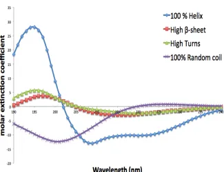
5 The different CD spectra that are produced by the various structures of chiral

molecules.4 . . . 40

6 The magnetic dipole transition moment, mexhibits circular motion, and the

electric dipole transition moment, µ, exhibits linear translation. These

(13)

7 A diagram of the optics that go into making a CD spectropolarimeter. It

contains a xenon arc lamp, mirrors, prisms, slits, polarisers, a lens, a PEM

and a PMT . The xenon lamp emits white light with a maximum flux in the

300 nm to 400 nm region. Mirrors direct the light to the slits and prisms.

Prisms select the relevant wavelength of light, polarisers perfect the linear

polarisation before the PEM makes it circularly polarised.5 _{. . . .} ₄₄

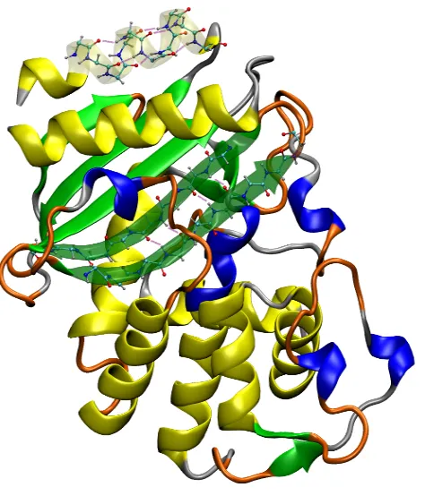
8 A picture of a protein with the different structures present: β−lactamase:

α−helix in yellow (long helices), 3-10 helix in blue (short helices), β−sheet

in green, turns in orange, random coil in grey. The atomic-scale detail, along

with hydrogen bonds, is also shown for two small sections: α-helix andβ-sheet

sections. The hydrogen bonds are the purple/pink lines between the red and

white atoms. Atoms are carbon in turquoise, hydrogen in white, oxygen in

red, and nitrogen in dark blue. . . 47

9 Figure from SOMCD paper showing that like proteins are clustered close

to-gether. The grey scales represent the Euclidean distances between nodes:

darker grey means the nodes are further apart. . . 56

10 A simple 2 dimensional representation of a transmembrane protein, E is

ex-tracellular space (outside the cell, which is an aqueous environment), P is the

plasma membrane (inside the membrane, which is a non-polar, phospholipid

environment, so it’s oily), I is the intracellular space (inside aqueous

environ-ment of the cell).7 _{. . . .} ₅₈

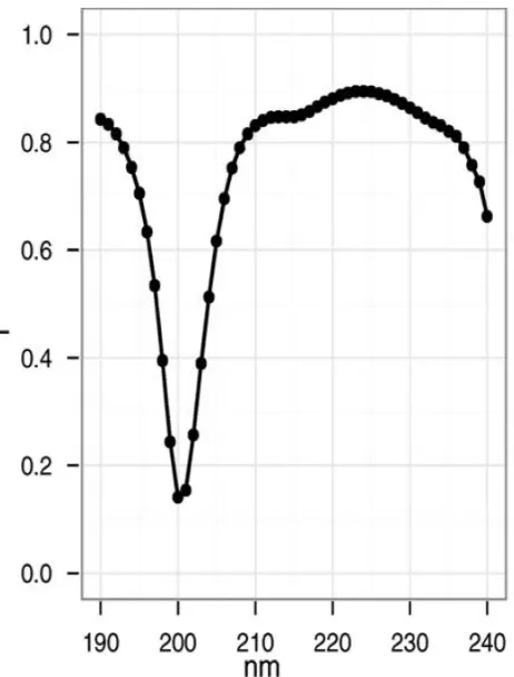
11 Plot from the K2D3 paper by Louis-Jeune et al. 2012 showing the Pearson

correlation coefficient against wavelength predicted by DichroCalc. . . 61

12 An annotated diagram of the intact human hand, by the American Society for

Surgery of the Hand.8 _{. . . .} ₆₆

(14)

5 List of equations

1. Euclidean distance ... Equation 1

2. RMSD ... Equation 2

3. NRMSD ... Equation 3

4. Learning rule ... Equation 4

5. Neighbourhood radius ... Equation 5

6. CD definition ... Equation 6

7. Absorbance ... Equation 7

8. Molar extinction ... Equation 8

9. Beer Lambert Law for ∆... Equation 9

10. Beer Lambert Law ... Equation 10

11. MRE Beer Lambert ... Equation 11

12. Mean residue ellipticity Beer Lambert ... Equation 12

(15)

6 Introduction

6.1 Self-organising map machine learning technique

As the rate of technological development increases more fields of research,

busi-ness, education, politics etc. have started and continued to produce prodigious

volumes of data. IBM estimated in 2012 that there were 2.5 exabytes (one

ex-abyte is 1018 _{bytes) of data created every day}10_{, and this will only keep}

accelerat-ing. Actually research shows that technology and scientific knowledge have been

growing exponentially for some time, and it is increasing this acceleration.11 _This

leads to the conclusion that what is needed is constant development of better

tools to manage the ever-growing data.

To that end we need to be sure that the software and hardware we use can

constantly grow its abilities for producing meaningful results, and that we have

enough data scientists, data analysts, software engineers and I.T. people applied

to the task. IBM estimates the world will need 4.4 million data scientists by

2015, and this will only be 1_/

3 filled.10

One of the fields that could greatly benefit from more automation of the

understanding of the information coming in from machines is the Biophysical

Chemistry work of circular dichroism (CD) spectroscopy. CD uses polarised UV

light to determine the conformation of certain molecules (proteins, DNA etc.)

be-fore, during and after chemical reactions, or other changes in the environment of

these molecules. This work aids in understanding the function of these molecules,

which helps with understanding biology, designing new medicines, and making

(16)

The research done in this project had the initial aim of developing something

that would help Chemistry researchers understand proteins, and make their work

easier, faster, and more accurate by becoming a sort of circular dichroism expert

software agent. This software, called SSNN for Secondary Structure Neural

Net-work, was designed to do pattern recognition on the CD spectra. The desired

outcome was for SSNN to learn what spectral features in the CD spectra lead to

which amounts of which secondary structures in the molecules. Though this is

not shown to users, it is just understood by the software.

The initial aim was to help CD practitioners by developing a software

ap-plication to learn about CD, however, the software developed with this aim has

grown far beyond that to include: finding the healthiest, comfortable insoles

for diabetes sufferers; controlling robotic prosthetic arms and hands, and even

matching Chemistry academics for research projects. CD, myoelectric signals

for robotic limb-control and diabetes was done by the author, the matching of

Chemistry academic primary investogators was done by Alison Rodger. This

software is now packaged in a graphical user interface (GUI), along with a guide,

so that anyone may download it from the Rodger Group website and use it on

their dataset.

As a machine learning method (see section 6.1.8), SSNN, the key software

package developed in this work, can be applied to any data set. It is the type of

software that will work on unlabelled data, where very little or no prior

knowl-edge is present (data mining). SSNN is a self-organising map artificial neural

network, or simply SOM, the SOM technique was invented by Teuvo Kohonen

(17)

Ko-honen Map. The acronym SOM is used to refer to an algorithm that constructs

an organised map, and the map itself. Hence the term self-organising map; it is

auto-organised. The self-organising map algorithm is a data-analysis technique

that works automatically, in an unsupervised manner.

This approach was employed to estimate structures (or conformations) of

proteins using circular dichroism (CD) spectroscopy, and later to control robotic

prosthetic limbs by performing the pattern recognition stage of interpreting

my-oelectric signals (MES) from patients.

This work focuses on unsupervised learning, and the SOM/SOFM or Kohonen

Map. The SOM places features of the dataset on its map in a way that enables

the user to gain knowledge about the features present, and their relationships

with other features, from the location on the map.13 _{The way the SOM is}

organ-ised to cluster data and display it in a 2 dimensional form helps one to easily get

an impression of what the topographical relationships between elements of the

data are, especially high-dimensional data that is very hard to picture or make

clear, quick conclusions about.

In summary, a SOM takes input vectors and generates a clustered map

rep-resentation of them, with interpolations. The interpolations are calculated as

a weighted sum of the few nearest nodes that best represent the experimental

vectors; these nearest nodes are called the best matching units, or BMUs. These

BMUs are closest in Euclidean distance. The Euclidean distance depends on

(18)

d=

v u u t

n X

i=1

(xi−x0i)2 (1)

where x is the observed datum in the input vector at position i, and x’ is the

calculated or theoretical value of it from the model generated by the SOM. Lower

case n is the number of elements in the input vector.

For the complete training of a SOM, the following is repeated for thousands

of iterations:

1. A CD spectrum (another input) is selected at random from the database

or reference set, and compared with the map to find a BMU (Figure 1).

2. The BMU on the map is made more similar to the input vector.

3. The neighbours of the BMU are updated too (Figure 2).

Through this process the SOM makes an organised map, or a clustered map of

input vectors. Similar vectors should be close to each other, and dissimilar ones

further apart. See Figure 1 for a view of how inputs correspond to the nodes of

a SOM.

Figure 2 shows the neighbourhood of a BMU is selected for learning as well,

while the rest of the map remains static for this iteration. This is how the

clus-tering works, if it does not make the BMU neighbourhood similar to the BMU,

then there will never be regions where certain classes of vectors are clustered,

(19)

Figure 1: Schematic illustration of a SOM. Each input vector is presented to the map, and each node comes to represent an input vector, or the interpolation between inputs. This assignment is completed by the time training has finished.2

See Figure 3, for an example of what one level of a SOM looks like once the

data it holds have been clustered. There is one level for each dimension of the

data space. The red, higher areas represent the regions of the data space that

have more positive values at this, the nth _{element of each input vector. Note how}

each value has been located amongst its equals or near equals. However, there

are still two areas with larger negative values: the low region in the front–left,

and the very low region in the front right. This shows that they belong to input

vectors that are of two different types. The other elements of the input vectors

(those not in this layer) place them in different classes, even if the elements on this

layer are similar. This is because there are far more relationships between data

points in the vectors present than just this layer, so they have a much stronger

influence on the organisation of the SOM than the elements of vectors that are

(20)

[image:20.612.209.465.276.523.2]

(21)

[image:21.612.202.463.158.363.2]

Figure 3: The trained SOM. The example here is a view of one level of a SOM that has clustered CD spectra; this represents the light intensities at one wavelength. Note how the terrain undulates smoothly, forming clusters: hills and valleys.

6.1.1 Origins of SOM

SOM is similar to the simpler, older methodology called VQ, vector quantisation.

The operation VQ performs is to compress and map continuous or discrete data

for transmission or storage in a digital channel. Vector-valued input data space

is segmented into a number of adjacent regions. A single model represents each

region optimally (a single point on the map). This is called the codebook vector.

In a SOM the equivalents of codebook vectors become globally ordered in space

(22)

6.1.2 Training a SOM

There are two ways to train a SOM 1) stochastically selecting individual examples

from the dataset, or 2) batch training, by considering all reference set examples in

one batch, and all models are updated simultaneously in a single step.

Stochas-tic training needs at least a few thousand training iterations to make sure all

examples from the reference set have had a good chance to have their impact

on the map. Batch training only requires a few dozen iterations before training

is complete, this is because a batch will typically contain many individual

vec-tors, so one iteration represents many from a stochastic training point of view.

Batch training is usually quicker and more likely to converge. Batch training does

not require any learning-rate parameter either (see sub subsection 6.1.6). The

stochastic training requires two learning-rate parameters, L0, the initial learning

rate, and k1, the rate at which learning decelerates. L0should be a small number,

in this work 0.06 or occasionally 0.1 were used. This ensures the algorithm learns

a bit each iteration, if the L0 were 1.0, then a node would become exactly the

training set spectrum in one iteration. This is not idea for clustering, it doesn’t

come to as good a convergence as slower learning. The k1 parameter should be

very small, as it multiplies the exponential in the learning rule equation, and

learning is needed throughout training.

6.1.3 Validating a SOM

One reasonably reliable way to validate the training parameters is to use

leave-one-out cross-validation (LOOCV). Here the SOM is trained with all but one of

the training set vectors, and tested on the vector that was left out of training.

(23)

of the map, the learning rate, the number of BMUs that go into making the

model, the learning equation parameters t1 and k1, and others. This is detailed

in “Paper 1”.17

6.1.4 Applications

Applications of SOM for clustering data are wide and include exploratory data

analysis, control systems, telecommunications, finance, natural science, statistical

analysis, biomedical analyses, profiling of criminal behaviour, characterisation of

galaxies, categorisation of real estate, and linguistics/organisation of texts.18–23

Some of the largest applications are bioinformatics, and huge textual databases.

In 2012, Kohonen et al. found over 10,000 applications of SOM14_. _Besides

SOM, there are other artificial neural networks, and there are many other

ar-chitectures, including evolutionary programs, artificial immune systems, random

(24)

6.1.5 Good practice with SOMs

The distance metric to measure the distances between data vectors on the map

needs to be decided upon. This could be Euclidean or more generally Minkowski,

Euclidean distance being Minkowski in 2 dimensions.14

The SOM is usually a square or hexagonal array of nodes containing the data

vectors. The square array is easier to build, and the hexagonal is better for

vi-sualisation purposes. It has been suggested that one should use a cyclic array,

such as a toroidal or spherical shape so that the edges of the map loop around

and become contiguous with each other. This is because there can be irregular

spacing between adjacent models at the extreme edges of the map. This format

is only suitable if the data itself is cyclic in some way.14–16,24

The size of a SOM should be large enough to include models for all spectra

or data vectors in the reference set, and to extract fine features of the data. So

if the data are expected to contain many fine features, a large map should be

used, otherwise the size should not be very large to optimise computational time.

The best way to establish the optimum size is trial-and-error. Typical sizes are

in the order of a few dozen to a few hundred nodes, and the dimensions of an

array should approximate the two principal components of the input data. Some

suggest using 4 to 10 nodes per expected class in the dataset.25 _{However, this}

should be validated by training a map of a particular size, and comparing its

results with results of maps of different sizes.

To initialise a large map, it may be advisable to train a small map, initialised

with the principal components, then once trained to a partially complete state, to

(25)

from the existing nodes. After that the larger map is trained until it reaches

acceptable clustering.14

When searching for the BMU for any reference or test vector in general, one

may save a great deal of computational time by taking note of the locations of the

previous BMUs, and the corresponding training data. In subsequent iterations

the search for the BMUs can be restricted to the vicinity of the previous winners.

This may also be done by pre-training a smaller map first: the approximate

regions of likely BMUs can be given to the large map. So if a cluster of one class

of data (Class 1) is found in the top, right corner, and another cluster of different

class of data (Class 2) is found in the opposite corner, then it can be assumed

that these two clusters will be in opposite corners of any map with the same

data. Training a larger map with these data should then proceed by only looking

for BMUs in opposite corners for these inputs when they are selected. One can

search only in the top, right corner for BMUs for class 1 input, then that corner

will be trained on that class 1. Later, when Class 2 data requires a BMU corner,

the bottom, left corner could be assigned to that. This is manually biasing the

larger map, so injecting knowledge, but that knowledge comes from the earlier

clustering with the smaller map.

Another method to speed up computation, and reduce memory requirements

is to truncate the data vectors:14 for example, selecting every fifth element in

the vector can reduce computation by a factor of 5, without losing many of the

features.

On may also select features one thinks are important in each input vector,

and then make a new dataset, where the first column is Feature 1, column 2 is

(26)

while hopefully keeping most of the important information. Features used should

be theoretically sound, and should be tested to determine if they lead to good

predictions, if there is a desired outcome.

6.1.6 SOM applied to circular dichroism spectra

In our methodology, SSNN, the spectra are clustered in an unsupervised manner,

but the protein secondary structures corresponding to these spectra are known,

so the algorithm can be improved until a certain level of accuracy is attained.

This is done by running the software many times (validation, usually LOOCV)

while varying the iteration count. An error metric that is useful in this effort is

the normalised root mean squared deviation, or NRMSD. The formula for it is

the same as the root mean squared deviation divided by the range of the observed

data:

RM SD=

r P

(xi−x0i)2

n (2)

and

N RM SD= RM SD

xmax−xmin

(3)

where for the CD data, xi is an element of the experimental circular dichroism,

CD, spectrum; xi’ is the estimation of xi from the predicted spectrum; n is the

number of elements in the spectrum (for example, for us this was 51 due to the

range of CD data wavelengths: 240 nm-190 nm); xmax and xmin are the

maxi-mum and minimaxi-mum of the observed values. The NRMSD is used in Dichroweb to

compare the CD analysis methodologies or algorithms available for use on that

website. On Dichroweb, each methodology used produces an NRMSD for the

(27)

test CD spectrum.

When testing many different SOMs with various numbers of iterations, using

a LOOCV test, the SOM arrangement with the smallest NRMSD for the test

spectrum in question is considered to have the best number of iterations.

A summary of how a SOM works is that one starts with a map, a collection

of random vectors arranged in an NxN square or hexagonal lattice. This map

comes to represent the data. This will be expanded with much greater detail later.

In our case we made a 40x40 square map of CD spectra. So the map in 3

dimensions is 40x40x51. Various sizes of map were tested, this was the best,

as is detailed in Paper 1.17 _{The value of 40x40 nodes in the SOM trained with}

our then 48 CD spectra was arrived at by running LOOCV for various map

sizes. It was found that a larger map size generally produced smaller error, but

larger than 40x40 nodes did not improve the accuracy much, and took a lot more

computational and real time to train. We found that this very large map, with 5

or 6 BMUs to make the model spectra from produced models with elements from

each of the BMUs: different regions of the spectrum were ’inherited’ from the

BMUs. If this were a simple classification question, then having a small map with

very few models might have been successful, but we were looking for 6 numbers

adding to 1.00 for the 6 different structure types, and the sets are not boolean,

but fuzzy. So for the most part each protein contained non-zero values for all 6

structures in varying amounts. The reference or training dataset also contained

these, and the test set did not contain any of the same spectra, so the structure

results should not be the exact structures of one model spectrum. Also, when a

small map is being used, making a model out of several BMUs tends to result in

(28)

in the map. For example, having a map with 9 nodes, and using 6 of those

to make the model of the test spectrum (6 BMUs) would be illogical, because

the model would be very average every time, there would not be much room for

individuality, and making a different decision (structure vector) each time.

The 48 spectra were later expanded to 53. We added 2 theoretically 100 %

α-helix proteins, by taking two helix spectra and stretching the peaks until they were where a protein of 100 % helix would be. We added 3 truly 100 % random

coil protein spectra. We present the map with the reference set of 53 CD spectra

in the sequential, stochastic manner detailed above. SSNN selects a spectrum,

and tries to find a match for it on the map. Each vector on the map is compared

with the selected CD spectrum, and the most similar one is said to be the BMU.

A learning rule (equation 4) makes the random vector more similar to the CD

spectrum. The region around the vector or BMU on the map, the

neighbour-hood, is made more similar to the CD spectrum by a smaller amount: decreasing

toward the edge of the neighbourhood (Figure 2).

The SOM architecture is used by some other methodologies for determining

protein secondary structure from circular dichroism, e.g. the K2d family26–28_{, and}

SOMCD13. The SOM is a good artificial neural network, ANN, for CD spectra,

as it allows one to see the clustering of the spectra without too much difficulty,

as each node of a SOM trained with CD spectra contains a spectrum; the SOM

is topological. The SOM is not the only ANN that might be used for pattern

recognition of CD spectra, but the visualisation capabilities do make it appealing

for such work.

After the SOM has clustered the CD spectra so similar spectra are close, it

(29)

These structures come from X-ray crystallography data. SSNN makes a map of

structures that correspond to the spectra by finding the CD spectra in the map

that are most similar to the reference set spectra. There are also many spectra

that are intermediate between the training set BMUs, and these are referred to

here as virtual spectra. These virtual spectra number (40x40 - 53 = 1547), more

of this is covered in Paper 1.17

Briefly, the 53 training or reference set spectra take up 53 nodes on the map,

the other 1547 nodes hold spectra intermediate between those. These are virtual

spectra, and are hybrids made from the elements from their training set

neigh-bours.

During the training process, learning proceeds so as to cause the SOM to learn

fast at the beginning, and exponentially slower towards the end of training. The

size of the neighbourhood is also reduced in size with iterations. The equation

for the learning is:

L(t) = L0·exp(−k1·t) (4)

where L is learning rate, L0 is the initial learning rate, t is the current iteration,

and k1 is a parameter of size<<1. According to Kohonen,14the learning rate of

the nodes should decrease monotonically (e.g. hyperbolically, exponentially, or

piecewise linearly) with iterations.

The equation for the neighbourhood radius is as follows:

radius(t) =



 

 

(RADIU S0−1)·(1− _tt₁) + 1 if t≤t1

1 if t>t1

(5)

where RADIU S0 is the initial radius of the neighbourhood, t1 is a parameter

(30)

According to Kohonen, the first 1000 or so steps of training the SOM should be

for ordering the map topologically, the rest of the time should be spent carefully

ordering the models to reach their best states. This may take 10 times longer

than the initial topological ordering stage.14

6.1.7 Developments to SOM

Fritzke 199429 _{made a self-organising network inspired by Kohonen’s SOM that}

adds more cells or nodes with iterations, i.e. “Growing Cell Structures”. There

are a few main differences between this and the SOM approach:

1. The learning or adaptation parameter remains fixed, while in a SOM it

reduces monotonically.

2. Only the BMU and its direct topological neighbours are updated to become

more similar to the relevant input vector, not a whole region.

3. Cells can also be removed

Removal of a cell can happen when the cell is considered superfluous, i.e. if it

has a position in a region of the data space with very low probability density; lower

than a threshold. The removal causes there to be fewer connections between cells,

and there can even be separate clusters with no links to each other, see Figure 4.

This method works using Voronoi regions, or regions created using Voronoi

tessellation.30,31_{Voronoi regions result from clustering data, such that every point}

in a Voronoi region of a Voronoi diagram is closer to the centre of each region than

any other centre. The centre of a region is called the seed, or centroid, and the

(31)

[image:31.612.220.457.271.530.2]

(32)

and an alternate name is Dirichlet tessellation, after Peter G. L. Dirichlet.30,31

The map is made of k-dimensional hypertetrahedrons, which look like

tri-angles when plotted in 2-dimensions. So the deletion of cells or nodes must

always leave behind connections forming hypertetrahedrons (in high dimensions,

or tetrahedrons in 3-dimensions, or triangles in 2-dimensions), rather than just

lines connecting free-floating nodes. The connection lines, or edges represent

neighbourhood relationships.29,30_{One advantage of using this ‘growing cell}

struc-ture’ methodology is that it makes obvious separation between different classes,

as there are no connections between nodes of different classes, due to deletion of

cells (nodes).

Fritzke et al. gave an example of classifying animals using the frequency cell

approach, with data taken from a SOM paper by Ritter and Kohonen.29,32 _The

SOM classified the animals correctly, but borders between the different classes

(bird, herbivorous quadruped, carnivorous quadruped) had to be drawn in by a

human, while the self-organising growing cell structure of Fritze classified

cor-rectly, and showed the boundaries automatically (projected in 2-dimensions).

In 1997 Kohonen et al. developed a SOM algorithm for signal processing

called ASSOM, or adaptive subspace SOM.33 In ASSOM, each node of the map

adapts to become an expert for one class of transformations. ASSOM makes

statistical representations that refer to various temporal events. As a member of

the SOM family of algorithms, it works by competitive learning, where there is

only 1 winner. This is in contrast to PCA, for example, which finds average data

features that come from global properties that are not temporal.

(33)

recog-nising patterns that are simple transformations such as rotation, scaling, and

translation. Examples they looked at were speech waveforms, and coloured noise

patterns from photographic images. ASSOM was successful in finding relevant

filters.33

6.1.8 General good practice in machine learning

SOM is a neural network type of machine learning; this section describes what

machine learning is, and how best to use it.

Machine learning is the branch of computing that deals with software that

can adapt its models to datasets; it learns from the data to produce more

accu-rate predictions. There are two main types of machine learning: supervised (for

labelled data) and unsupervised (for unlabelled data). An additional method is

reinforcement learning, described just below.34

In supervised learning, the algorithm is given the input vectors, and their

target vectors, so that, during training, it may perfect its patterns to replicate

those targets/predictions. Examples of supervised learning include multilayer

perceptrons (MLPs), and genetic algorithms (GAs) with definite goals.29

In unsupervised learning, the algorithm will study the data, and find

pat-terns that are previously unknown. This process includes clustering, for example

SOM, hidden Markov models (HMM), and GAs with open-ended goals. SOM

is an unsupervised, competitive learning method.14,29,35 _{The ability to use}

unla-belled data makes unsupervised learning useful for data mining, where the truth

(34)

because no human can understand the data, as they are far too high dimensional,

so there can be no correction of the predictions.

There is also reinforcement learning, which is a method of programming

soft-ware agents using rewards and punishments, while not requiring an explanation of

how to perform a given task. The agent must learn using trial-and-error methods

in a dynamic environment. The two main ways to solve reinforcement problems

are 1) to search for a behaviour that performs well in the environment, and use it

(GAs and GP), and 2) to estimate the usefulness of taking actions in the

environ-ment by using statistical techniques and dynamic programming techniques.36,37

The basic goal of all machine learning, ML, techniques is to gain the ability

to generalise to much more than just the training set. This is because the ML

system will never be able to have all information about every possible situation,

however, just having vast amounts of data does not suffice to be able to generalise

well. Like a brain needs to be able to learn new knowledge, because instinct will

never give it the ability to cope with every possible situation in a changing world.

If we give a ML system a Boolean function (two possible correct answers for

each variable: true or false) with a moderate 100 dimensions, and one million

examples in the sample data, this would mean that there would be 2100 - 106

ex-amples with unknown classes, i.e. approximately 1030 _{unknown classes. The way}

to solve this problem, or set of problems, is to include some knowledge or at least

assumptions along with the raw data. 100-dimensional data is easily reached,

the circular dichroism spectroscopy data we work with is 57 dimensional, and the

(35)

Wolpert gave a name to the problem of having to include knowledge, rather

than just data, to make better learners. He called this ‘no free lunch’ theorem,

meaning that, when trying to understand all functions that are needed in the

universe, on average no learner may do better than guessing randomly. In this

sense there is no difference between algorithms without knowledge.39–41 No

al-gorithm can predict everything in the universe. It will need some knowledge to

be better than another prediction algorithm that has no knowledge, just data.

This may lead to the problem of having to supply vast amounts of data to train

the algorithm, assuming the functions that describe the patterns in a given data

space are uniformly distributed.

Fortunately, the functions that describe the samples are not taken uniformly

from all possible mathematical functions. Assuming the following: that similar

examples will have similar class membership, that the functions will be smooth,

and that complexity is finite, are all in the set of few assumptions that are

suffi-cient to understand rather well.

When learners use induction, a little input knowledge can be transformed into

a lot of output knowledge. It is superior to deduction in that it requires a much

smaller supply of knowledge to show good results.41 _{However, it was always}

be-lieved that with inductive reasoning the correct decisions and causations cannot

be guaranteed, unlike with deductive reasoning, where they can be. More recently

this has been found to be untrue; there can be guarantees on results gained from

inductive reasoning, especially when accepting probabilistic guarantees.41

In any machine learning methodology, before beginning the training, the data

(36)

classifier may a) learn the data well, b) have its parameters and architecture

val-idated, and c) be tested on a new dataset. The testing phase is needed so it may

show that it can make general conclusions about data, and is not over-trained

on specific data. This cannot really be done when the answers are not known, as

can be the case with data mining.

Having the test dataset enables one to answer the question of how accurately

the classifier needs to predict the target vectors; too little training, and the

algo-rithm does not know the data, and has not recognised any patterns (underfitting),

too much training on the specific training set, and the algorithm cannot

gener-alise (overfitting).41

Underfitting is where a learning or heuristic algorithm has not been trained

enough to recognise patterns in the dataset, and so cannot make good

predic-tions or classificapredic-tions for this or any dataset. Overfitting is where a heuristic

algorithm has trained too much on one particular dataset, and believes that is

all there is to know, so it cannot predict or classify any new data well. It keeps

assuming the new data is exactly the same as, or very similar to the training data

set.41

One can understand the problem of overfitting by dividing the error of

gen-eralisation into two parts: bias and variance.42 _{Bias is learning the wrong thing}

consistently, and variance is caused by a tendency to learn random things, and

not the true information.

There are various ways to work against overfitting. Cross-validation can help,

(37)

terms added to the evaluation function are also a good idea, like penalizing the

size of classifiers so that they do not get too large and have space to overfit.

The next biggest problem for machine learning is “the curse of

dimension-ality”. As dimensions (or number of features) of the data grow, generalising

becomes exponentially more difficult. If the number of features in the database

is again just 100 with a Boolean solution space (two options: true or false), and

even as many as 1012 _{samples are given to the classifier algorithm, the samples}

still only cover 10−18 of the input space (2100 ≈1030).

A more deep-rooted and important issue is that the way ML algorithms

clas-sify based on similarity fails in high dimensions. When there are 100 dimensions,

and only 2 are being compared, the noise from the other 98 dimensions can act

as noise, and can drown-out the signals from the first 2.14

So is gathering more features always a good thing? No, it can be that they

offer nothing new that is not already known, and their pros can be outweighed

by their cons, when they contribute to there being too many dimensions to the

features. Assuming the examples are uniformly distributed, then the detriments

to having more data become much worse quickly. Actually, the situation is not

as bad as it may seem, as examples are not usually spread uniformly, but cluster

about the lower-dimensions.14

In success or failure of ML techniques the most vital element is that the

features used are good. When dealing with raw data, learning is not

straight-forward. However, if one forms good features from the raw data, learning can

(38)

the ML algorithm takes raw data, it will find pattern recognition far more

dif-ficult than if it works with data that has had some important features highlighted.

Machine learning is an iterative process of 1) applying the data or features

to the learning algorithm, 2) analysing the results, 3) altering the algorithm and

maybe the data. Here learning is usually the easy stage (ML algorithms have

general application, so easily learn data), while feature engineering is the most

difficult stage, as it is domain-specific. Automating feature engineering to an

increasing degree is therefore a very worthy pursuit. This could be done by

cre-ating a large collection of features that might be useful and picking those that

help best to improve classification information.

Despite all of the above, an algorithm with vast amounts of data still wins

over a better classifier with much less, which of course might lead to computation

time issues.41

There were no computation time issues for the CD project, as the dataset

that trained the selected ML technique, the SOM, was 57 by 53 data (points),

from 57 dimensions and 53 examples. As mentioned above, the aim was to take

the CD spectra and structure knowledge, and do some pattern recognition on

them to find spectral features that link the spectra to the secondary structures.

The question was: what features lead to what structures of proteins, and in

what proportions? Aspects of the history of this field of work, along with some

(39)

6.2 Circular Dichroism for protein secondary structure

estimation

Circular dichroism, CD, is a spectroscopy that has been used since the 1960s

in structural biology to study the structures of peptides, polypeptides and

pro-teins.43

CD was discovered in the 19th century by Jean-Baptiste Biot, Augustin

Fres-nel, and Aim´e Cotton.44 _{CD is the difference in absorption of left- and}

right-circularly-polarised light (LCP light minus RCP light), see the equation below5

∆A=AL−AR (6)

where ∆A is the difference in light absorbed by the chiral molecule, and AL

and AR are the absorptions for the LCP, and the RCP light respectively.

Absorbance is the logarithm of the incident divided by the transmitted

radi-ation, as in the equation below:

A=log10(

I0

I ) (7)

where A is absorbance, I0 is the incident radiation, and I is the transmitted

ra-diation.45–47

In order for a CD spectrum to produce a useful, non-zero signal, the molecules

have to be in a suitable solution (known as a buffer), and the molecule must have

some chirality (explained just below). A buffer is a solution that resists changes in

acidity, so if a small amount of acid or a base is added to the buffer solution that

(40)

approxi-that is being used. A chiral molecule cannot be superposed onto its mirror image,

the arrangement in space is very similar, but not exactly the same, just in the

same way that a left and a right hand are not arranged in exactly the same way,

and are not simply reflections of each other. CD is based on the Cotton Effect

or Optical Rotatory Dispersion, which is where the biased absorption between

LCP and RCP light by stereoisomers of a chiral molecule causes redistribution of

electrons in a helical way, for certain transitions, at particular wavelengths. By

studying the CD spectrum of a chiral molecule, the handedness of the changes in

electron positions can be found. Some aspects of the structure of the molecule in

three dimensions can be derived from this.43,48 _{Stereoisomers are molecules that}

have the same atoms and sequence, but different spatial arrangements.49,50

The basis of the CD spectrum is electronic transitions, this gives rise to

spec-tral features: peaks and negative bands. In Figure 5, we can see the CD specspec-tral

features that arise from the structures present in a chiral molecule. α-helices have a characteristic large peak at about 190 nm, and two negative bands at 208

nm (called the π →π∗ transition) and 222 nm (n →π∗ transition). β-sheets are characterised by a peak between 195 nm and 202 nm (π→π∗ transition), and a negative band between 215 nm and 220 nm. Turns are negative at 180 nm to 190

nm, and positive at 200 nm to 205 nm. A disordered structure has a negative

band at 200 nm. These are for the same set of electronic transitions, they just

shift in wavelength a little for different structure types.

Electronic transitions involve electrons jumping energy levels near the ground

(41)

[image:41.612.174.499.140.390.2]

Figure 5: The different CD spectra that are produced by the various structures of chiral

molecules.4

CD can be measured in terms of molar extinction coefficients, or ∆, also called molar absorptivity, which has the units L mol−1 _cm−1_:

∆=L−R (8)

and

∆ = ∆A

cl (9)

whereL andR are the molar extinction coefficients for the LCP and RCP light,

c is the concentration of the chiral molecule in solution measured in mol·l−1_{, and}

I is the cell pathlength, measured in centimetres. The pathlength is the width

(42)

passes through.

We worked with ∆ values, which are per mol, so our data are independent of the number of residues. Equation 9 is derived from Beer Lambert’s Law:5

A=cl (10)

∆ values can be converted to mean residue ellipticity (MRE or θ) using the simple equation:

θ = ∆∗3298.2 (11)

MRE is measured in degrees cm2 _dmol−1 _residue−1_{. CD spectrophotometers}

output the CD signal in units called millidegrees. This is because, historically,

the change in polarisation of linearly polarised light into elliptically polarised

light passing through the sample was measured as the CD signal. Millidegrees

can be converted into ∆ units using the equation below:

θ/millidegrees = 32,982·cl (12)

which is the Beer Lambert Law (equation 10) restated for different units.5

LCP light is defined as: when viewed from the source, the electromagnetic

field of LCP light rotates in an anti-clockwise direction, and the EM field of a

beam of RCP light rotates in a clockwise direction.51

6.2.1 Where CD signals come from

Circularly polarised light has a magnetic dipole moment that rotates (a magnetic

(43)

motion of the electromagnetic field. The helical motion of the EM field causes

an electron to move in a helical path, as can be seen in Figure 6.5,6

Figure 6: The magnetic dipole transition moment,mexhibits circular motion, and the electric dipole transition moment,µ, exhibits linear translation. These combine to make helical motion of the EM field.5,6

So the EM field moves in a helical motion, but how do CD practitioners find

the signals these helical motions of light produce? The CD machine, which is

called a spectrophotometer or spectropolarimeter records the CD spectra. An

extremely important part of a circular dichroism spectropolarimeter is the

com-ponent that makes sure the machine produces exactly equal intensities of both

LCP and RCP light. This component is the PEM, or photoelastic modulator.

The UV light source is a xenon arc lamp, which also emits visible light. Various

mirrors, prisms and slits are needed to collimate the light from the lamp.

Subse-quently, the light is linearly polarised (as would be useful for linear dichroism),

and the PEM circularly polarises the light.

The PEM is made of crystalline quartz stuck to a piece of isotropic quartz

(sil-ica). Light travels through the silica section. The light is split into two orthogonal

(44)

dif-section of the PEM, this makes it oscillate at 50 kHz. Varying the amplitude

of the voltage causes the PEM to select alternately for light polarised in one

direction, followed by the orthogonally polarised light.

So the PEM effectively forms a wavelength-dependent quarter-wave plate that

is needed to make circularly polarised light. In Figure 7, see a diagram of the

optics of a CD spectrophotometer (another name for a CD machine). The PMT

(photomultiplier tube) detects the light that was not absorbed by the sample,

and converts it to an electrical signal; it vastly multiplies the current received,

and is a very sensitive detector.

The CD signal is then determined by the ratio of the AC to DC elements

detected by the PMT, see equation 13. The sign of the CD derives from the

phase of the AC element using a lock-in amplifier that uses the AC voltage of the

PEM as a time reference.5,36

CD = < AC >

DC (13)

Instruments can now hold the DC current constant, with the use of a servo that

adjusts the PEM voltage. With a constant DC voltage, the CD is proportional

to the <AC> voltage.

6.2.2 Buffers

To perform CD analysis of chiral molecules, an appropriate buffer should be used.

A buffer is a solution containing a weak base and its conjugate acid, or a weak

acid and its conjugate base. The purpose of a buffer is to resist changes in pH

when small amounts of acid or base is put in it52_{. A buffer should be at a}

concen-tration in the solution such that it may withstand variations in the pH due to the

addition of a highly charged ligand, for example ATP4−_{. The buffer must be used}

(45)

[image:45.612.215.482.289.495.2]

(46)

constant. The pH should be checked at the temperature the buffer will be used

at; some buffers have high temperature coefficients.53,54

Buffers can affect the CD spectra when they are used for solutions of proteins

or other chiral molecules. Every time a CD spectrum is taken of a chiral molecule,

the base line should also be scanned. This is the CD spectrum without the chiral

molecule present, i.e. just the buffer solution. This should then be subtracted

from the CD spectrum for the molecule of interest to obtain the true spectrum.

This should also be done to check the quality of the buffer, as some can cause

the high tension, HT, voltage to rise to a level where the CD spectrum becomes

too noisy to be useful. This is due to the buffer having a high absorbance in this

wavelength range. The high tension voltage is the voltage applied to the PMT.

Absorbance in a CD spectrum due to the buffer solution can cause degradation

of the signal, to the point that the signal to noise ratio becomes too low. Kellyet

al.53 _{found that absorbance is wavelength dependent, and more noise is caused}

at short wavelengths, particularly the 190 - 200 nm region. The absorbance is

measured by the HT voltage. This is the voltage applied to the photomultiplier

tube (PMT). This means the PMT has to work hard in the short wavelength

region. For good CD spectra the HT should be at most 600 V, but this depends

on the CD machine.53

For this reason synchrotron light sources with much greater light fluxes than

xenon arc lamps are used to gather what is termed SRCD, or synchrotron

ra-diation CD. With a synchrotron, useable CD spectra can currently be obtained

down to approximately 160 nm. However, due to noise from most desktop CD

(47)

nm.

Unwarranted interactions, like chelation (the formation or presence of bonds

between separate binding sites on the same ligand and one central atom) of

essential metal ions can also cause trouble with phosphate buffers among others.53

6.2.3 Algorithms for circular dichroism pattern recognition

With knowledge of where the CD signals come from, and how to prepare the

buffer, the data analysis stage needs to be considered, as the CD spectra are

not easily read by non-expert CD practitioners. Despite being able to tell which

structures are present, even the experts cannot say exactly what proportions of

structures are present. For this statistical or learning algorithms should be used.

There are various methodologies for CD pattern recognition to find secondary

structures of proteins: CDSSTR, SELCON3, VARSLC, CONTIN, LINCOMB,

MLR, CDNN, SOMCD, K2d, K2D2, K2D3, as well as our own: SSNN.13,26–28,55–57

Here is a brief review of the methods used. SELCON3, CDSSTR and K2d were

tested and reviewed in attached papers. The methodologies are based on

multi-ple linear regression (MLR), singular value decomposition (VARSLC, SELCON,

CDSSTR), ridge regression(CONTIN), convex constraint analysis (CCA),

self-consistent method (SELCON), constrained least squares analysis (LINCOMB),

and neural network (CDNN, SOMCD, K2d, K2D2, K2D3, SSNN).58 The

struc-tures for these databases generally come from X-ray crystallography. See Figure

(48)

[image:48.612.228.465.241.518.2]

(49)

Greenfield’s review

In reference58 _{Greenfield compared the structure prediction qualities of MLR,}

LINCOMB, SVD, CCA, CONTIN, SELCON, B¨ohm et al.’s NN, and K2d.

Most of the algorithms are good at predicting the α-helix structures from CD, but have more difficulty with all other structures. The helix structures were

predicted by all algorithms with Pearson correlation coefficients (P) of 0.88 or

higher, and standard deviations (σ) of usually about 0.1. Theβ-sheet andβ-turn structures were not as well done, and were far more variable. β-sheets were pre-dicted with P of 0.00 to 0.91, and σ of 0.07 to 0.28. Theβ-turns were predicted with P values of -0.56 to 0.84, and standard deviations of 0.05 to 0.27.

K2d does not predict the structure type β-turns, it uses the structure types 1) α-helix, 2) β-sheet and 3) other.26,58

MLR (non-constrained least squares analysis) predicts α-helix, β-sheet parallel and anti-parallel, β-turns, and random conformations.

LINCOMB predictsα-helix, β-sheets, β-turns, and “random coils”. B¨ohm et al.’s neural network predicted helix, parallel and anti-parallel sheet, turns, and

remainder.

A likely reason these algorithms predict β-turns so poorly is because there are at least 4 different types of turns, which do not have very similar spectral

features associated with them.

MLR predicts helix well, sheet with some correlation with experimental, and

turns very poorly. Similar to MLR, LINCOMB predicts helix well, sheet with

some correlation (very variable), and turns rather badly.

SVD predicts helical structures very well, but sheets and turns extremely

(50)

0.12 ≤ σ ≤ 0.27, and turns -0.56 ≤ P ≤ 0.22, and 0.1 ≤ σ ≤ 0.27. Here P is Pearson’s correlation coefficient, and σ is the standard deviation. So a large P, closer to 1.00, is better (higher correlation), and a small σ is good (small error). CCA makes good predictions of helical structure, but its estimates of sheets

and turns are worse than that of other methods.58

CONTIN gives good helix predictions, and its turns predictions are better

than MLR, SVD and CCA. VARSLC produces excellent helical structure

pre-dictions, while sheet and turn predictions are much improved over the above,

especially the sheet predictions. Data needs to be collected to 184 nm to make

useful predictions/estimations, which is a handicap.58–60

SELCON’s predictions for globular protein helix, sheet and turns are all very

good. There does not seem to be much detriment to using a reduced data range of

240 nm - 200 nm. The 1996 version of SELCON worked well for globular proteins,

but did not predict well the structures of polypeptide with large percentages of

sheet; it over-estimated helix content, while under-estimating sheet content quite

badly. For a comparison between SELCON3, a more recent version of SELCON,

and SSNN see Paper 117 and Paper 34.

The Neural Network for protein secondary structure estimation that was

writ-ten by B¨ohm et al. was extremely good at predicting helical, and antiparallel

sheet structures. The correlation coefficients were 1.0 and 0.91. The only

prob-lem appears to be when the wavelength is restricted to 250 nm - 200 nm, the

sheet estimation is negatively correlated.61

K2d gives good sheet estimates when the wavelength range is restricted. It does

not estimate turns.

(51)

nm - 200 nm, VARSLC uses the range 260 nm - 184 nm, and SELCON uses

260 nm - 200 nm. B¨ohm’s NN (neural network) used 83 element input vectors,

representing the intensities at 260 nm - 178 nm.58 MLR does not require an exact

value of the protein concentration. According to Greenfield, CCA does not find

the secondary structures of unknown proteins easily, given no extra information,

but it is very good for analysis of spectra of proteins and peptides with regard to

temperature, pH and ligand binding.

MLR, SVD and CCA do not have selection procedures for known spectra

to make model spectra of unknown proteins. The known spectra do not

neces-sarily have similar features to the test spectra. This leads to the models being

very dependent on the spectra which were chosen to make the models. So, the

suggestion was to introduce these similarity selection measures. That is what

has been done with (1) ridge regression, (2) variable selection, and (3) neural

networks; examples of these are (1) CONTIN, (2) VARSLC (which is SVD with

variable selection) and SELCON (VARLSC modified), and (3) K2d. Algorithms

with selection perform better than those without. SELCON, or self-consistent

method by Sreerama and Woody gains a speed advantage by routinely removing

the spectra least like the test spectrum.58,62–64

It should be noted that the algorithms that produce the best spectral

predic-tions do not necessarily produce the best structure estimates. Greenfield points

to CONTIN as “almost always [giving] excellent agreement between the

experi-mental and calculated CD curves, even when the fits are relatively poor compared

to other methods.” Greenfield says that K2D often produces very poor spectral

models, while making very good structure predictions.58 _{Another example of this}

(52)

CD-to-protein-structure algorithms, but its structure predictions/estimations are not as

good as some competitors (e.g. SELCON3 and SSNN). SELCON3 has possibly

the best structure predictions besides SSNN.58

The most sensible way to analyse CD spectra to get structure predictions is

to use at least a few different methods, and see where they agree. If the

predic-tions vary greatly, then one cannot have great confidence about the structures

present.4,58

Greenfield says that if one needs structure predictions, but does not know the

concentration accurately, then non-constrained least-squares analysis programs

like MLR are the only options, but these do not give the best predictions. This

issue is dealt with in reference38 _{also known as Paper 2 in this thesis.}

K2d

In their 1993 paper, Andrade et al. introduce K2d, their SOM methodology

for estimating protein secondary structures from CD spectra.26 This paper lends

more detail about K2d and its proteinotopic map, than given by Greenfield,

mentioned above. A proteinotopic map is a topological map of some information

about proteins.

The training set for the K2d SOM is 24 CD spectra. One of these proteins is

poly-L-lysine, which has different CD spectra depending on pH and temperature;

for this reason it is used as a model protein for the various spectral features.

Eighteen of the proteins have known (static) structures, and 3 are constructed

from 15 proteins of known structure originating from Chang et al. 1978.65 More

(53)

The K2d map is a 13x13 square lattice of nodes and, like other SOMs, it

in-terpolates between experimental CD spectra, but does not extrapolate. For this

reason, unlike some methodologies, K2d does not give structure estimates with

negative values, which would be physically impossible.

As Unneberget al.13_{point out, the database size determines the possible sizes}

of the map: a map needs to have enough data space to store all the examples,

but must not be so large as to make all BMUs in a region essentially the same,

and negate the use of multiple BMUs. That would cause the SOM to produce

poor spectra models. So with 24 spectra in its training set, K2d needs a smaller

map than a SOM with more spectra would.

Due to the CD data used by K2d being of the wavelength range 240 - 200 nm,

there are 41 data points. The SOM does not use CD spectral data beyond 240

nm, as there is not much information from the peptide backbone in that region.

For reasons of wavelength range and how much information can be extracted

from such a range, there are 3 structures types estimated by K2d, α-helix, β -sheet and “random coil”, or other. There are not enough electronics transitions

that emit light in this region to provide information to resolve more thanα-helix

and β-sheet. The n → π∗ transitions are between 190 nm and 200 nm. This

means that there are only 2 independent variables, for the helix and sheet; the

random coil value is calculated by subtracting the helix and sheet values from

1.00.26 It should be pointed out that random coil is a particular structure type,

though rather difficult to generate, but is often used as a category for everything

that does not fit into any other categories, like the group “other” structures.

(54)

to the structure of the protein, or other chiral molecule, in the short-wavelength

range below 200 nm. However, this data is much harder to access due to the

high energies required, and most desktop CD spectrophotometers cannot get CD

spectra in this range without increasing the absorbance to such levels that there

is a great deal of noise (at the time of writing, May 2014).

As mentioned above, this is a reason to use SRCD, the synchrotron overcomes

this absorbance issue, see the section on SRCD, section 6.2.4.

Some later algorithms inspired by K2d do use data in the 200 - 190 nm range.

The Andrade team point out that while collecting spectra without the shorter

wavelength region, the methodology cannot hope to reliably estimate multiple β

structures, hence why they decided to estimate just one helix structure and one

sheet structure.

K2d uses a parameter to track the training progression of the SOM, it is

called the distortion parameter, D. D is the sum of all the distances between

each training set spectrum and the model spectrum most similar to it. If this

value is generally decreasing, then training is headed in the right direction. If

it stalls, and does not continue decreasing, then training has stopped being useful.

With regard to the success of clustering CD spectra, the K2d SOM team

found that each of the three structure labels claimed a corner of the map; in the

random coil corner, those spectra of proteins with high random coil clustered,

with the same result for sheet- and helix-rich proteins.

K2d uses a BMU count of 2. This is the number of BMUs, or model spectra

from the map that go into making the final output model of the test spectrum,

Self organising map machine learning approach to pattern recognition for protein secondary structures and robotic limb control

Self Organising Map Machine Learning Approach

to Pattern Recognition for Protein Secondary

Structures and Robotic Limb Control

Vincent Austin Hall

Contents

1

Acknowledgments

2

Declarations

3

Abstract

4

Abbreviations

List of Figures

5

List of equations

6

Introduction

6.1

Self-organising map machine learning technique

6.2

Circular Dichroism for protein secondary structure

estimation