Automating system generation in Clash

(1)

1

Faculty of Electrical Engineering,

Mathematics & Computer Science

Automating System Generation

in C

λ

ash

Erik van Raalte [s1879383] Master thesis

March 12, 2019

Exam committee:

(2)

(3)

Summary

There is an increased interest in graduation assignments that involve the usage of the Cλ

ash-language. To prevent that obtained knowledge in these projects is neglected, the CAES chair started a project where multiple students will work on a framework in the Cλash-language

that can be utilized for real-time systems. This thesis is written in the early stages of the project. The ability to enable the communication of the (to be created) functional blocks is considered important and should be defined in an early stage of the project. The research question was therefore defined as: How can the unique features of the Cλash language

be utilized to define a deterministic System on Chip interconnection standard? This Master thesis proposes a methodology and presents a tool that generates hardware from data flow.

In the background, several alternatives to derive a communication structure on a chip are discussed or excogitated. A conventional SoC communication standard is considered as a useful asset, as it enables to quickly derive a working system in a relatively short amount of time. It is also possible to create a deterministic system, if a simple bus architecture with a static schedule is used. However, implementing a conventional SoC standard does not utilize the properties that the Cλash-language offers. The quick realisation of a

pro-totype is also not set as a requirement. After this conclusion, the Cλash-language was

extensively applied a variety of different approaches. Along the way, several limitations are found. In the end, the proposed approaches are compared in a Design Space Exploration (DSE). From the DSE is concluded that a method that enables generation of hardware from a data flow graph and a so called dependency graph is the most interesting option to work out.

In the realisation phase, the data flow to hardware methodology is carefully defined. There-after, the methodology is implemented in Haskell and the Cλash-language. In the

implemen-tation phase, various limiimplemen-tations of the Cλash-language are found, which resulted in certain

design choices for the presented data flow to hardware tool. The supported data flow model is HSDF, but it should not be difficult to support a subset of SDF. In the end, the tool is put to test with two design examples.

(4)

for the tested examples, because the tool mainly concerned the scheduling of the functional blocks and not the generation. Furthermore, the definition of a system on a higher level likely introduced overhead. Moreover, synthesis involves compiling the source to a supported (undecipherable) HDL with the Cλash-compiler, and synthesis from the generated HDL to the

hardware. In one of the examples, the used synthesis tool could not work with the generated Verilog, while VHDL did not result in any problems. Therefore, bugs and compatibility of the Cλash-compiler can be a liability for the continuation of the project. Another major

limitation was that Cλash is very strict with data types. It was opted to automate the nesting

(5)

List of acronyms

IC Integrated Circuit

HDL Hardware Description Language

VHDL VHSIC Hardware Description Language FPGA Field Programmable Gate Array

CAES Computer Architecture for Embedded Systems LUT Look Up Table

RTL Register Transfer Level P2P Peer to Peer

HDL Hardware Description Language SoC System on Chip

CPU Central Processing Unit GPU Graphics Processing Unit

ASIC Application Specific Integrated Circuit IP Intellectual Property

AXI Advanced eXtensible Interface

AMBA Advanced Microcontroller Bus Architecture AHB Advanced High-performance Bus

APB Advanced Peripheral Bus

TCP/IP Transmission Control Protocol / Internet Protocol DSE Design Space Exploration

RTS2 Real-Time Systems 2

HSDF Homogeneous Synchronous Data Flow (MR)SDF (Multi-Rate) Synchronous Data Flow CSDF Cyclo-Static Data Flow

FIFO First-In First-Out

(6)

(7)

Introduction

A System on Chip (SoC) combines several electronic building blocks to a single chip as an (complex) electronic system. As opposed to conventional systems where components are connected with external wires, the components in a SoC are all internally connected as an Integrated Circuit (IC). This allows the designer to create physically smaller circuits that use less power and achieve a higher operating speed. A Central Processing Unit (CPU) or Graphics Processing Unit (GPU) is a SoC that is designed as an Application Specific Integrated Circuit (ASIC). These integrated circuits are fast, energy efficient and relatively cheap in large quantities. A system is described in an Hardware Description Language (HDL) such as VHSIC Hardware Description Language (VHDL) or Verilog. A cell libary with the available gates and corresponding characteristics is required to synthesize the description to an integrated circuit. Unfortunately, prototyping a system on an ASIC is relatively expensive, since the functionality of the chip cannot be adjusted after the manufacturing process. This is where the Field Programmable Gate Array (FPGA) is advantageous over the ASIC.

An FPGA is technically an ASIC that consists of many reconfigurable logic blocks with functionality that can be set by the designer after the chip has been manufactured. A block is often called a Look Up Table (LUT). These LUTs can be set to several combinational functions or used as memory. The logic blocks can also be inter-wired, providing design freedom. The functionality of an FPGA is described using methods similar to ASIC design. The main difference is that the description is translated to a bitstream using the software that is supplied by the manufacturer, and then programmed on to the FPGA.

During the last decades, the number of LUTs in FPGA’s has grown significantly, and this subsequently resulted in an increase in the market size. Still, even though there is more hardware that can be described in the collection of logic cells, the languages did not follow the same trend of growth. Compared to all high level programming languages, Verilog and especially VHDL can feel cumbersome. Starting in 2009, the Computer Architecture for Embedded Systems (CAES) chair within the University of Twente has developed the Cλ

ash-language, which uses a functional approach to describe hardware. The Cλash-language is

(12)

Cλash-language code to VHDL or Verilog, that can by synthesized to an FPGA or ASIC.

Nowadays Cλash is developed further by the spin-off company Qbaylogic. However, the

language is still taught on the university as part of the Embedded Computer Architectures 2 course. It is also possible to do a graduation project that involves the usage of Cλash.

Unfortunately, the CAES chair noticed that a lot of the results of existing master projects were often neglected in new projects. In March ’18 the chair started a project in which multiple students participate and can apply their Cλash knowledge in order to design and refine a

robot platform that has a Xilinx Zybo Z7 backbone. One of the aspects in which the CAES chair wants to distinguish itself from the Robotics and Mechatronics chair on the University, is that it wants the robot to operate real-time and be deterministic. The Cλash-language is a

functional and therefore pure language. It’s properties could be useful in designing such a system.

Real-time systems is one of the main research fields within the CAES chair. The con-cept ”real-time” is used in many contexts. In the context of this thesis, a system is real-time if the exact behaviour can be characterized for all possible inputs and states that might occur. In other words, it should be deterministic.

1.1 Problem description

When several students work on their own sub-system or Intellectual Property (IP) blocks within the robot platform, it is of great significance that there is a communication standard in the early stages of the project. Especially if these components rely on information from each other. This Master project aims to resolve this necessity. The research topic during this project is defined as: How can the unique features of the Cλash language be utilized to define a deterministic System on Chip interconnection standard?

1.2 Outline of this thesis

This section describes the path that was taken throughout this project. In Part I, The back-ground of the research is presented. The backback-ground consists of four chapters. In Chapter 2, the fundamentals of the Cλash-language and compiler are discussed. The remaining

chapters discusses several approaches to realise communication on FPGAs.

The first approach is discussed in Chapter 3. In this chapter, the characteristics of existing protocols that are used to communicate on FPGA systems are presented and compared, it concludes with the rudimental demonstration of the Wishbone standard in Cλash. The

second approach is listed in Chapter 4. It describes attempts to optimize conventional FPGA communication by using properties of the Cλash-language. The third approach (Chapter 5)

(13)

chapter discusses the fundamentals of data flow models and proposes how the model can relate to hardware designs. Then, the proposed approaches are compared to each other in the Design Space Exploration (DSE) that is listed in Chapter 6. The approach from Chapter 5 was considered the most the most valuable.

(14)

(15)

Part I

(16)

(17)

Chapter 2

C

λ

ash

The purpose of this chapter is to provide the reader with some of the fundamentals of The Cλash-language and compiler. Although some parts are quite comphrehensible for those

new to functional programming, other parts are more advanced. For this reason, all examples are accompanied by a diagram that depicts what the code actually does on a hardware level. The Cλash website explains clearly why one could use the Cλash-language for hardware

description [1]:

The Cλash-language is a functional hardware description language that borrows both its

syn-tax and semantics from the functional programming language Haskell. It provides a familiar structural design approach to both combinational and synchronous sequential circuits. The

Cλash-compiler transforms these high-level descriptions to low-level synthesizable VHDL,

Verilog, or SystemVerilog.

2.1 Fundamentals

The Cλash-language implements a subset of the Haskell functions, and adds additional

functionality for digital circuit design. Generating a synchronous (updated on the rising edge of the clock) function from a pure (without internal state) combinatorial function can be accomplished with amealy,mooreorregisterfunction. The simplified data type declaration

of a mealy machine is as following:

mealy :: (s->i->(s,o)) -> s -> Signal i -> Signal o

The first argument of themealyfunction, is a function with data types that must comply to

a specific form, namely: (s->i->(s,o)). It has the current state of data type s and the

input of data type ias input, and it produces a tuple consisting of the next state of data

typesand an output of data type o. Furthermore, the internal state, which should be of

the data types, has an initial value that is given as the second argument of themealyfunction.

Themealyfunction converts the combinatorial function, to a block that can capture state. It

(18)

is a pure language without internal state. Therefore, variables in the discrete time domain are packed in theSignaldata type, which is represented as a infinitely long stream of states of

that variable. The variables are ”updated” on the rising edge of the clock that is defined in the system. This is the reason the last argument (the input), and the return value of the mealy machine (the output) are both of theSignaldata type.

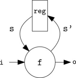
A basic example is shown in Listing 1 and depicted as hardware in Figure 2.1. The function

f(line 1-4) adds the inputiand current states, and assigns as the new states’(line 3).

The current state is assigned to the output (line 4). The mealy machine is constructed in thetopEntityfunction (line 6-7). Functionf, which has the required form, is given as first

argument. The initial state (the value0) is assigned as the initial register value in the second

argument. The topEntity is the function that the Cλash-compiler compiles to an HDL.

Dependencies of thetopEntityfunction are compiled as well. The data type declaration of

the top entity must be monomorphic (exist in only one form), in order to be compiled to an HDL. In this example aSigned 6data type is used.

1 f s i = (s',o)

2 where

3 s' = s + i

4 o = s

5

6 topEntity :: Signal (Signed 6) -> Signal (Signed 6)

7 topEntity = mealy f 0

Listing 1: Mealy machine example

reg

i

_f

o

[image:18.595.221.348.467.596.2]

s’

s

Figure 2.1: The mealy machine

2.2 Higher Order Functions

The aforementioned example shows how combinatorial logic like an adder can be used in a synchronous manner within the mealy machine. Another aspect that makes Haskell and the Cλash-language powerful are the Higher Order Functions (HOFs). HOFs are functions

within functions. For example thefoldlfunction:

(19)

Thefoldlfirst takes a function (e.g. an arithmetic operation) that takes two data types (b

anda) and produces a result ofb. The next argument is the initial value of data typeband

the last argument is a vector of data typea. The result is a value of data typeb. The structure

of afoldlis depicted in Figure 2.2 and Listing 2. The initial valueais applied with the first

entry of the vectorxsto the functionf. The result of this operation is passed as argument for

the second instance off, along with the second record of the vectorxs. This continues until

the end of the vector is reached and the answer is computed. Note that this HoF is still purely combinatorial.

f xs!!0

f xs!!1

f xs!!2

a b

Figure 2.2:Visualization of thefoldlfunction

1 b :: (b -> a -> b) -> b -> Vec n a -> b

2 b f a xs = foldl f a xs

Listing 2:foldldeclaration

If the vectorxsis fairly large, then the functionfis replicated more often. Despite that the

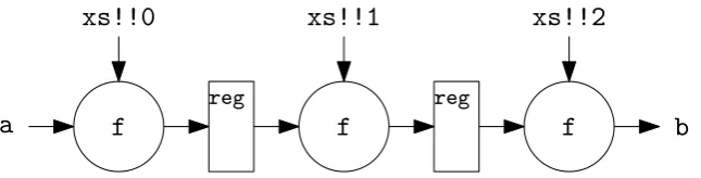
functional description is still correct, it might result in trouble when the algorithm is mapped on an FPGA, due to the larger area and longer critical path. The functional correct expression can be rewritten to be advantagous in terms of speed or area. Figure 2.3 and Listing 3 depict a version of thefoldlwith registers between the instantiations of the functionf. As a result,

this circuit has a shorter critical path. The function is no longer purely combinatorial, and requires a description that involves the mealy machine that was discussed in Section 2.1. First a function calledbTis described. It has a form such that it can be used as an argument

of the mealy function.

Line 1-7 lists the constraints that the function bT must comply to. It has the structure

where inputs are shifted through a set of registers, where the functionfis applied to the

intermediate results. The fieldsrsandrs’hold the current and next state of the registers

(line 8). Line 11 is the most interesting for this example. First, the inputais shifted into the

vector of registers that hold the current state (a +>> rs). The next state of the vector (rs’), is

described as functionfexecuted over both (a +>> rs) andxs. This is accomplished by the zipWithfunction. Line 14-18 describes the data type definitions of the mealy machine and

line 19 describes the initialization of the mealy machine. The first argument is the function

(bT (1:>2:>3:>Nil) (+)), which complies with input requirement of the mealy machine,

see Section 2.1. The second argument is the initial state of the registers, which are all set to

(20)

f

xs!!0

f

xs!!1

f

xs!!2

a

b

[image:20.595.126.449.84.166.2]

reg reg

Figure 2.3:Visualization of a pipelined instance of thefoldlfunction

1 bT

2 :: KnownNat n

3 => Vec (n+1) a

4 -> (a->a->a)

5 -> Vec (n+1) a

6 -> a

7 -> (Vec (n+1) a,a)

8 bT xs f rs a = (rs',o)

9 where

10 o = last rs'

11 rs' = zipWith f (a +>> rs) xs

12

13 -- Initialisation:

14 b

15 :: HiddenClockReset domain gated synchronous

16 => Num a

17 => Signal domain a

18 -> Signal domain a

19 b = mealy (bT (1:>2:>3:>Nil) (+)) (repeat 0)

Listing 3: Foldl optimized for throughput by means of pipelining

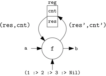
Figure 2.4 and Listing 4 show an instance of the foldl that is optimized for size. As opposed to the pipelined version, where the functions are chained after each other, this version used a self loop. This approach can be more efficient in area usage, because it uses only two variables to hold the current state, and only one instantiation of the functionf. However, it will

not produce a valid output on every clock edge. It therefore has a lower throughput than the pipelined instance. AgainbT(line 1-12) is in a form, such that it can be supplied as argument

to the instantiation of the mealy machine (line 15-20). Instead of applying the function f

on the intermediate values that are contained in the vector of registers, there is only one function and one register that contains the intermediate result. On line 11, the new value of the intermediate result is assigned. It only fetches the input when a state counter has reached the maximum value, otherwise it processes the intermediate result. An additional register that holds the value of the counter, that is used to monitor the state of the intermediate value (line 10). The output only holds the result when the counter has reached the maximum, otherwise it holds0(line 12). This implementation is flawed, because there is no distinct signalling of

the validity of the output signal. A solution is addressed in Section 2.4. In conclusion, the Cλash-language allows the designer to first focus on the algorithm, and then on the mapping

(21)

reg

cnt

res

(1 :> 2 :> 3 :> Nil)

a f b

[image:21.595.221.405.85.216.2]

(res’,cnt’) (res,cnt)

Figure 2.4:Visualization of a small area instance of thefoldlfunction

1 bT

2 :: (KnownNat n, Num a)

3 => Vec n a

4 -> (a->a->a)

5 -> (Int,a)

6 -> a

7 -> ((Int,a),a)

8 bT xs f (cnt,res) a = ((cnt',res'),o)

9 where

10 cnt' = if cnt == length xs - 1 then 1 else cnt + 1

11 res' = if cnt == length xs - 1 then f a (xs !! 0) else f res (xs !! cnt)

12 o = if cnt == length xs - 1 then res' else 0

13

15 b

17 => Num a

18 => Signal domain a

19 -> Signal domain a

20 b = mealy (bT (1:>2:>3:>Nil) (+)) (0,0)

Listing 4: Foldl optimized for area consumption, without status signals

2.3 REPL and simulation

Another useful aspect of the Cλash-language, is the ability to simulate every expression in an

interactive environment calledclashi. This makes it tangible to evaluate a system consisting

of multiple expressions seperately. After the whole system is simulated inclashi, it can be

compiled to a synthesizable HDL, a testbench for Vivado or Modelsim can automatically be generated as well. The resulting simulation should have the same behaviour as theclashi

simulation. A common practice is to first define the system in the Cλash-language and

simulate it in theclashienvironment and then generate the testbench to simulate it with the

tools provided by the FPGA supplier.

2.4 Algebraic data types

The last aspect of the Cλash-language that is discussed in this chapter are the algebraic

(22)

results of functions. A basic data type is theBooldata type, which is monomorphic (can only

exist in one form), because it’s representation is unambiguous:

1 data Bool = False | True

An instance of Bool can be either True or False. There are also data types that take a

parameter and therefore exist in more than one form, for example the polymorphic (which means that it can exist in multiple forms)Maybedata type:

1 data Maybe a = Nothing | Just a

Within this data type,acan be any data type (e.g.IntorString), butNothingwill always be Nothing. It is useful in functions that do not produce a result at all times. It can for instance be

applied to improve the example that was depicted in Figure 2.4. The improved code is shown in Listing 5. The example is more complex and only the crucial differences are discussed. Instead of just inputs and outputs of the data typea, this example has wrappedain theMaybe

data type. For the input holds, as long as it isNothing, no new value is fetched. A value of Just afetches the valueaand resets the counter. The output in this example isNothing, as

long as it is not valid, otherwise it isJust <result>. The initialization of the mealy machine

in line 20-25 is changed, as the input and output are of theSignal domain (Maybe a)data

type.

1 bT

2 :: (KnownNat n, Num a)

3 => Vec n a

4 -> (a -> a -> a)

5 -> (Int,a)

6 -> Maybe a

7 -> ((Int,a),Maybe a)

8 bT xs f (cnt,res) a = ((cnt',res'),o)

9 where

10 (cnt',res',o) =

11 case a of

12 Just r -> (1,f r (xs !! 0), Nothing)

13 Nothing ->

14 if cnt == length xs - 1 then

15 (0,f res (xs !! cnt),Just res')

16 else

17 (cnt+1,f res (xs !! cnt),Nothing)

18

20 b

22 => Num a

23 => Signal domain (Maybe a)

24 -> Signal domain (Maybe a)

25 b = mealy (bT (1:>2:>3:>Nil) (+)) (0,0)

Listing 5: Foldl optimized for area consumption withMaybedata type

Data types can also be created by the designer. By pattern matching on the data type, an elementary arithmetic logic unit can be created in a few lines of code, see Listing 6. The executed function depends on the first argument, which is of the Operatordata type that

(23)

belong the theNumclass. It produces a result that is of data typeaas well (line 4). E.g. alu Add 1 2executes the function on line 5, andalu CmpGt 1 2executes the function on line 9.

1 data Operator = Add | Sub | Incr | Imm | CmpGt

2 deriving (Eq,Show)

3

4 alu :: (Num a) => Operator -> a -> a -> a

5 alu Add x y = x + y

6 alu Sub x y = x - y

7 alu Incr x _ = x + 1

8 alu Imm x _ = x

9 alu CmpGt x y =, if x > y then 1 else 0

Listing 6: Arithmetic Logic Unit in the Cλash-language

In conclusion, there are many additional options that the Cλash-language provides in contrast

to conventional languages like VHDL and Verilog. The next chapters explain the process on how to utilize the Cλash-language and compiler on conventional SoC communication

standards, as well as new approaches to enable SoC communication. In the remainder of this thesis, both the Cλash-language and Cλash-compiler are designated under the name

(24)

(25)

Chapter 3

Comparison between existing SoC

communication standards

The aim of this chapter is to understand the basic concepts of commonly used communica-tion protocols in the industry. The full study on existing SoC communicacommunica-tion standards is presented in Appendix A.

There exist several interfacing protocols for Systems on Chips. The provided IP blocks for Xilinx FPGA’s are for example connected through the Advanced eXtensible Interface (AXI) [2] from ARM. The standard Intel Altera FPGA peripherals communicate over the Avalon bus [3]. Other common protocols are the Advanced Microcontroller Bus Architecture (AMBA) [4] from ARM and the Wishbone bus [5] from Opencores. This chapter concerns a comparison and overview of common features and methodologies used in existing SoC protocols. More elaboration on the individual protocols can be found in Appendix A.

The protocols that are described in Appendix A feature some common practices. The only communication standard that is entirely different is the network on a chip methodology, which is only briefly discussed in this chapter and not in the appendix.

3.1 Characteristics of existing communication standards

(26)

[image:26.595.184.386.239.387.2]

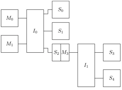
It is common that a bus consists of master and slave interfaces. An IP that is connected to a master interface, may initiate transfers to an IP that is connected to a slave interface. A slave interface does in general not initiate a transfer, and just responds to a master. A bus consist of a group of masters and slaves that can communicate by means of an interconnect, see Figure 3.1. The mastersM0 andM1may communicate with slaves S0,S1 andS2. If every

master had a connection to every slave, that would results in many wires. An interconnect is a device which directs communication between masters and slaves, by routing them together, and thus saving wires and energy.

M0 M1 S0 S1 S2 I0 I1 S3 S4 M3

Figure 3.1:An example bus topology

There exist several types of interconnects. One interconnect type is a shared bus, as is used in the AMBA protocol. In a shared bus, all masters and slaves are connected together, see Figure 3.2a. Since only one instance may communicate over the interconnect at the time, an arbiter that directs the communication is required to make this work. Another approach is a so called crossbar interconnect, which creates a physical connection between a master and a slave, so that multiple masters can communicate with a different slave, at the same time, see Figure 3.2b. The latter has the advantage that it can provide a higher throughput since masters can simultaneously communicate with slaves. However, it has a larger hardware utilization.

M0

M1

S0

S1

S2 S3

S4

M3 Shared bus

Arbiter A0

A1

(a)Shared bus interconnect

M0

M1

S0

S1

S2 S3

S4

M3

Cross bar

Arbiter A0

A1

[image:26.595.64.506.583.744.2]

(b)Crossbar interconnect

(27)

There are also types of communication that do not involve an interconnect. One of them is so called Peer to Peer (P2P) communication where a master interface is directly connected to a slave interface. A chain of P2P interfaces (an IP block can feature a slave and a master interface at the same time) is sometimes also referred to as a pipeline interface. These kind of interfaces are used when high datarates are required (for example image processing). Commonly used communication standards differ in the support of Master to Slave connection methods.

Another distinction is the protocol that is used to communicate. Every protocol uses a different set of signals to send and receive commands and data. The AMBA standard even offers two seperate interfaces that offer a different kind of communication (Advanced High-performance Bus (AHB) and Advanced Peripheral Bus (APB)). On a high level each communication protocol performs the same function namely, transfer data or request data, but the different implementations lead to different characteristics on both area and performance. Some protocols allow so called burst transfers, where a master does a single request and the slave responds in multiple words. Most protocols do also support embedded status messages about the transfers. This can be used to optimize the scheduling in the interconnect. For example, a slave is given a burst request and it can only give a part of the response. Then it can notify the master that it did not send the entire message yet. These are called split transfers. Many protocols also support pipelining, where a master can queue several requests at a slave, it therefore does not have to wait for a response to initiate a new request.

3.2 Network on a chip

(28)

[image:28.595.85.287.83.284.2]

Core Ni Core Ni Core Ni Core Ni Core Ni Core Ni Core Ni Core Ni Core Ni Core Ni Core Ni Core Ni Core Ni Core Ni Core Ni Core Ni Core Ni Core Ni Core Ni Ni S IP core Network Interface Switch Physical link S S S S S S S S S

Figure 3.3: A Network on a Chip architecture from [6]

3.3 Comparison

This study clarified the basic concepts of some SoC communication standards, along with a recent approach called Network on a Chip. The communication standards that are discussed with more comprehension in Appendix A, share some of the characteristics that were dis-cussed in Section 3.1. However, some standards are more complex then others. The FPGA architecture that is used is relevant in the choice of the communication standard as well. The Avalon standard is only used by Altera IP blocks. Therefore it would not make sense to use this standard in a Xilinx FPGA, as there are simply no IP blocks availible that comply to this standard. The Wishbone bus comes with a variety of open source packages that work on both Xilinx and Intel Altera FPGA’s [7]. Xilinx IP’s use the AXI4 bus, but the standard is very comprehensive to code by hand. Xilinx offers interface generation tools, but they do lack the support of code generation to Cλash. Finally, the Network on a Chip methodology is

considered overly complex for the application that is aimed to be build.

The Wishbone is likely the best choice if an existing standard is chosen. The protocol is simple and yet versatile as it supports a majority of the options that more complex proto-cols offer. A rudimentarily Wishbone master and slave are described in Appendix B of this thesis. Although the description is relatively simple, it does not utilize the unique properties of Cλash, like higher order functions. Therefore, the description is similar to a conventional

(29)

Chapter 4

Existing Communication optimized

with C

λ

ash

This chapter describes a part of the research that was done as after the implementation of the Wishbone master and slave (see Appendix B). Although the Wishbone master and slave worked as expected, it still required a large amount of manual labor to connect a set of slaves and masters to an interconnect. In an environment like Quartus or Vivado this is relatively easy to connect interfaces together, due to the availability of a block diagram editor and extensive support for conventional hardware description languages.

The aim of this chapter is, to find a method that inherits properties of existing SoC standards, while utilizing the properties of Cλash to connect components in a more elegant manner.

Moreover, it also investigates the possibilities to use algebraic datatypes to define a more intuitive communication protocol, as Cλash is less readable on bit level, opposed to Verilog

or VHDL due to the strict type system.

4.1 Assignment of slaves to an address space

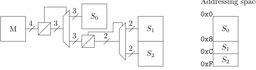
A master can communicate to slaves through an address space. An interconnect can either communicate the address the master requests to all slaves, where the slaves have to do the decoding, or use an interconnect that decodes the addresses. This is explained best through by means of an example:

• One master with 4 bit address space • One slave that has a 3 bit address space • Two Slaves with 2 bit address space

(30)

is shown in the left part of the figure. The most significant bit functions as a control bit for the subsequent multiplexer.

4

3

2

2 M

0x0

0xF

0x8

0xC

[image:30.595.64.498.133.252.2]

Addressing space

Figure 4.1: Hardware and address space allocation for the presented example

Ideally, one would specify a master with an accompanying addressing space, along with a list of slaves and their adressing space. The aim was to use Cλash to automatically

derive a interconnect architecture that would allocate the slaves within the addressing space. Unfortunately, after many attempts this turned out to be unfeasible mainly because it would require multiple slaves with varying address space as argument. This is not possible due to the semantics of the Cλash-language. The only solution that worked was to generate an

individual addressing filter for each slave. However, this creates a large amount of redundant hardware. For example, S1 and S2 in Figure 4.1 share the first multiplexer, this would be

replicated with the aforementioned filtering method. An alternative approach, that has not been worked out, is to outsource the address decoding to the slave itself and transfer the whole message from the master to all the slaves.

4.2 Communication with algebraic data types

Another approach that is attempted, is a communication standard that relies entirely on the algebraic datatypes. This method was neglected early when it turned out that it could not possibly result in an efficient Register Transfer Level (RTL) implementation. However, it is included to clarify the steps that have been taken within this master project.

The concept is to create slaves that utilize an unique instruction set. The master can then run the instructions that the slave supports directly. A rudimental example that controls the state of 4 LEDs is shown in Listing 7. TheOpCode andRspCode (line 5-6) data types

show the instructions and responses that the slave supports. The State data type (line

4) represents the data that is registered in the slave. The behaviour of the slave itself is defined inslaveT(line 8-14). Note that the type declaration is conform with a function that

can be supplied to a mealy machine. The slaveThas an internal state of type State as

first argument. The second argument (the input), is a value of the typeOpCode. The output

of the function is the the response to the master (RspCode) as well as the updated state

(31)

(Write State), read the current pattern in the LEDs (Read) or do nothing (OpIdle). In the

example that is considered in the next paragraph, another slave that controls an RGB LED is considered as well. The internals of this slave are similar to the earlier explained LED, and therefore not shown.

The master can communicate with both the slaves as shown in Listing 8. The data type

Slaves(line 1) contains all possible operation codes, as it is eitherLed Led.OpCodeorRgb Rgb.OpCode. The advantage of this method is that it does not require address decoding, as

the instruction set represents the addressed slave. A master could execute commands to both slaves as shown in line 3-8.

The problem with this method is that it gets inefficient on RTL level, as theSlavesdatatype

can get relatively large. Moreover, this design has a structure of a single core processor. The master is destined to act as a director within slaves, which will likely cause bottlenecks in larger use cases. Moreover, multiple instances of a slave require yet another operation code in theSlavestype. In conclusion, it is not scalable.

1 module Led where

2 import Clash.Prelude

3

4 type State = BitVector 4

5 data OpCode = Write State | Read | OpIdle

6 data RspCode = RspWriteOK | RspRead State | RspIdle

7

8 slaveT :: State -> OpCode -> (RspCode,State)

9 slaveT s i = (rsp,s')

10 where

11 (rsp,s') = case i of

12 (Write x) -> (RspWriteOK,x)

13 (Read) -> (RspRead s,s)

14 (OpIdle) -> (RspIdle,s)

Listing 7: A algebraic slave that controls 4 LED’s

1 data Slaves = Led Led.OpCode | Rgb Rgb.OpCode

2

3 prog :: [Slaves]

4 prog = [

5 Led (Led.Write 0b1000),

6 Led (Rgb.Write 0b010000),

7 Led Led.Read

8 ]

(32)

(33)

Chapter 5

Hardware and data flow

This chapter presents a method to derive an hardware architecture from a subset of syn-chronous data flow. The intention is to present the data flow fundamentals and explain why data flow can be useful in real-time applications. Subsequently, one of the studies of this thesis is presented. It describes how hardware could be derived from data flow.

5.1 Dataflow

The book that is used as part of the Real-Time Systems 2 (RTS2) course [8] on the University of Twente explains the fundamentals of Dataflow with full comprehension. This section only explains the part of the theory that is required to understand the material in this thesis.

Multi-core programming is often described as a difficult programming challenge. It is hard to reason about the utilization of parallelism while designing correct functional behaviour. The RTS2 course presents a model for multi-core systems and the tools to analyze these systems. Multi-core does not only refer to multi-core CPU’s, as it can also point to multi-accelerator systems, as often used in FPGA systems. The analysis model is called data flow and is explained in the next paragraph.

Dataflow is a set of models that can be used to describe real-time behaviour. In this thesis Homogeneous Synchronous Data Flow (HSDF)and Multi-rate Synchronous Data Flow (SDF) are considered. HSDF consists of the elements that are shown in Figure 5.1. A snippet from [8] gives the following definition of HSDF: A Homogeneous Synchronous Dataflow

(HSDF) is defined as a directed graphG(V, E) that consists of actorsv ⊆V and directed

edges withe⊆E withe= (vi, vj). The edges represent First-in-first-out queues that have

unbounded storage capacity. In the queues indivisible tokens can be stored. Homogeneous

(34)

v

0

[image:34.595.196.373.81.153.2]

Actor

Edge

Token

Figure 5.1: Elements of data flow

An actor is a node without state that can represent a task, such like a mathematical function. A task that is represented by an actor is executed when the actor fires. An actor within a HSDF graph must comply to a so called firing rule: one token must be present on each incoming edge of an actor. In multi-rate graphs, this can be more than one token as well. After an actor has fired, it produces a token (or multiple tokens in multi-rate) on all it’s outgoing edges. The time between the consumption of tokens on the incoming edges, and the production of tokens on the outgoing edges is called the firing duration. A token is a indivisable element, which means it can not be party consumed or produced. Due to the abstraction of the model, a token can present data, space or synchronization events. Tokens are distributed among actors by means of queue that is represented by an edge. Queues can hold an unbounded amount of tokens. Furthermore, tokens are consumed from a queue in the order that they are produced.

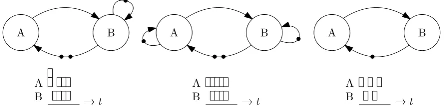
A graph consisting of the elements described above is called a HSDF graph. Because of the semantics, these graphs can by analyzed on throughput and latency. Another propery of data flow is that it is deterministic, which makes it useful for real-time applications. The designer must find a data flow model for the application that is designed. A correct model allows to be examined thorougly on utilization, throughput and latency. The analysis tech-niques themselves are not part of the scope of this thesis. Some examples of HSDF graphs are shown in Figure 5.2. An edge from an actor to itself is called a self edge. A self-edge forces an actor to fire non-concurrent. The graph on the left in Figure 5.2 does not feature a self edge at actor A, and the result is that it consumes and fires tokens concurently as shown in the schedule below the graph. The centered graph features self-edges on both edges, which prevents the concurrent firing. The graph on the right cannot fire concurrently due to insufficient tokens. In this thesis the self edges are implicitly added to the actors.

A B A B

A

B _→_t

A

B _→_t

A B

A

B _→_t

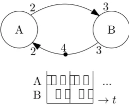
[image:34.595.63.507.632.743.2]

(35)

Another variation of synchronous data flow is (Multi-Rate) Synchronous Data Flow ((MR)SDF) [10] and is often called SDF. An rudimentary SDF graph is depicted in Figure 5.3. As the name suggests, it support multiple consumptions or production of tokens in comparison with HSDF. The cited literature gives a more comprehensive definition, this explanation serves only as a quick overview.

A B

A

B _→_t

4 2

2 3

3

[image:35.595.247.377.175.283.2]

...

Figure 5.3:SDF example, every actor has an execution time of one time unit and implicit self edges.

One other aspect that is concerned is the consistency of graphs and the repetition vector. The full theory on repetition vectors has been elaborated in Chapter 5 of [8] and proven in [10]. An SDF graph is called consistent if the production and consumption of tokens over time is balanced. An inconsistent graph causes the amount of tokens to increase towards infinity (unlimited buffers, not feasible), or decrease to zero (deadlock, no actor can fire). The consistency can be determined with the topology matrix that is shown in (5.1). The columns in the matrix represent in and outcoming edges the actors in a graph and the rows represent the edges that are present in the graph.. A consumption of an edgeekis labeled byγkand a

production is labeled byπk, see Figure 5.4.

Ψ =

"

π0 −γ0

−γ1 π1

#

(5.1)

-

γ

1

π

0

-

γ

0

π

₁

A

B

Figure 5.4:Graph that is represented by (5.1)

The topology matrix of the graph in Figure 5.3 is represented in (5.2). The repetition vector is the smallest integer vectorzsuch thatΨ~z=~0. If the graph is connected and consistent and after each actorvihas firedzi times, then the repetition vector indicates the number of firings

required of each actor, that result in the initial token state on the edges. For the matrix shown in (5.2) the repetition vector is~z=

"

3 2

#

(36)

order to return to the initial token distribution.

Ψ =

"

2 −3

−2 3

#

(5.2)

A data flow graph can fire either self-timed (fire as soon as the firing rules are obeyed) or according to a schedule (the firing rules are still obeyed, but the enabling time of an actor can vary). A graph where the actors eventually fire according to a reoccuring pattern is called periodic. Actors can also fire according to a strictly periodic schedule. A strictly periodic schedule has as additional constraint that each of the actors in a graph fire in a periodic schedule themselves. This can be clarified by the example that is shown in Figure 5.5. The lower schedule is periodic. The firing pattern repeats every three time units (A→A→B).

Therefore, the scheduled is called periodic. A schedule is strictly periodic if every actor in the schedule fires periodic with respect to itself ors(k) =si(0) +kpj. In the periodic schedule,

the time between firings with actor A varies between 1 and 2 time units. Therefore the actor does not meet the requirements for a periodic actor. The time between firing for actor B is always 2 time units, and therefore this actor is periodic.

A schedule where all individual actors fire periodic, and thus the schedule of the graph is strictly periodic, is shown in the upper part of Figure 5.5. It can be observed that the utilization of the actors is lower in the strictly periodic schedule.

A

B

A

B

t

A B

1

2

2 2

Periodic Strictly periodic

Figure 5.5: Difference between periodic and strictly periodic, implicit self edges and an execution time of one time unit for both actors are assumed

A method to efficiently derive the strictly periodic schedule of a given valid data flow graph is described in [11] and implemented in Haskell in [12].

5.2 Relation between data flow and hardware

(37)

As discussed in the introduction, defining hardware in functional languages can shorten the process from algorithm to hardware, as the definition of the algorithm and mapping the algorithm on hardware can be separated. The mapping flexibility that Cλash features can be

utilized to optimize an architecture for throughput, latency or power consumption in a later stage of the design process.

In Section 5.1 it was discussed that although the semantics of data flow are limited, it is a powerful tool to analyze systems on latency and throughput, and could therefore be suitable for real-time hardware design. One of the major limitations of data flow is that there is no choice element. Many existent hardware designs use decision making. It therefore is difficult to derive data flow from hardware that was designed in a conventional manner. An approach is to use abstractions in data flow. E.g. If an actor has an execution time of either 1 or 5 time-units, the actor can be modeled with an execution time of 5. This is pessimistic, but it assures that it can still be analyzed with data flow tools. However, this is just a trivial example where one actor is considered. if an existing hardware architecture results in a fairly large network of actors with variable execution time, abstraction gets more difficult and results in a less accurate representation of the system that is analyzed. A type of data flow graphs that covers varying execution times is called Cyclo-Static Data Flow (CSDF) [14].

The problem can also be approached the other way arround. In other words, hardware may also be derived from data flow instead. A basic data flow graph of the HSDF type is depicted in Figure 5.6.

A

B

Figure 5.6:A basic HSDF graph with two actors, self edges are implicit and the execution time of both A and B is one time unit

(38)

not represent a dependency of B on A. Another way to look at tokens is as an synchronization mechanism on the schedule where A and B comply to. E.g. If Figure 5.6 has an additional token on the edge from A to B, then both actors could fire simultaneously and the throughput would be different. However, the graph still holds no information about the dependencies on data between both actors. To resolve this problem, an additional graph as shown in Figure 5.7 can be introduced.

A

B

Figure 5.7:A graph that depicts that B has a dependency on A

The graph is called a data dependency graph and it consists of the actors that are present in an accompanying data flow graph, along with edges that only indicate data dependency between the actors. This concludes the system in which A and B are present: Both the scheduling and data relation are now derived.

From the information of both graphs a hardware architecture can be derived. But first the definition of tokens should be elaborated more. Another data flow schedule for which the data dependency in Figure 5.7 still holds, is shown in Figure 5.8. According to the graph, actor A firesN times as often as actor B. Therefore, the amount of tokens on the edge B

to A represents a First-In First-Out (FIFO) data buffer with sizeN, between A and B. The

definition of data flow states that edges represent an unbounded token capacity, but this is not feasible in a real design. From the distribution of tokens on the edges, it can be derived what data buffer sizes are required.

A

B

N

1

1 N

N

Figure 5.8: Another SDF graph. self edges are implicit and the execution time of both A and B is one time unit

In the aforementioned graph, A firesN times, then B fires once, after which the schedule

repeats. The designer could improve the throughput of the graph by increasing the buffer fromN toN+ 1. This adjustment causes that A does not have to wait for B to complete in

order to fire again, hence improves the throughput. The designer can also use SDF anal-ysis tools to detect deadlock occurence or other undesired behaviour, if the schedule is known.

(39)

(40)

(41)

Chapter 6

Design Space Exploration

The DSE is a systematic method to characterize alternatives to criteria. In this chapter the alternatives that are proposed in the background and characterized to the criteria that are proposed in the introduction. In summary, the communication standards must comply to the following requirements:

• The development language is fixed to the Cλash-language;

• The resulting structure should be deterministic.

The next paragraphs evaluate the three approaches that could be elaborated further during this research. The chapter concludes with a comparison of the presented approaches, and concludes with the approach that is realized.

A conventional SoC standard

One of the major advantages of using an existing SoC standard is that the implementation is just a matter of following the specification. Another advantage is that there are many IP’s that use these standards. Hence one can use existing IP’s and reduce the time until there is a functional platform. However, it is not important to create the robot platform as soon as possi-ble, since it has no commercial use. Another aspect is that all existing protocols operate on bit-level, simply because this is convenient in conventional languages. The Cλash-language

supports higher order functions, which may enable a fundamentally different design approach. Another downside of conventional standards is that they are designed for systems that are not neccesarily set up to be deterministic. Dataflow requires a static schedule in order to be fully deterministic. A conventional communication standard can also be deterministic if a static schedule is used, but does not offer advantages over the strict data flow methodology.

Communication using algebraic data types

Both Cλash and Haskell use a (customizable) data type mechanism. The proposed idea

(42)

look like RotateMotor 1 200 (Rotate motor one 200 degrees). However, tests with this

methodology result in inefficient structures on RTL level since there can not be a bus if every IP can use a different datatype to transfer data or instructions. It is not scalable to larger designs as well.

Data dependency & data flow approach

The approach presented in Chapter 5 with data dependency and data flow has the advantage that the hardware can systematically be derived from both the data flow (scheduling) and the data dependency (data). It also enables the hardware architect, to adjust the schedule at compile time (e.g. pre-evaluation in Haskell) in order to improve performance in different areas. It will therefore also use the properties of Cλash and Haskell. Moreover, it is a

fundamental different approach which is interesting for the CAES group. The downside is that the standard is non-existing and must be carefully defined. It will therefore likely take longer to create a functioning prototype.

6.1 Comparison and conclusion

The three proposed methods are evaluated on the constraints that were elaborated in the introduction of this chapter, and rewarded accordingly. The rewards are ranked on an ordinal scale: −<0 <+. The weights on each constraint are equal. Therefore the total score is

the sum of all the constraints. The highest scoring approach is elaborated as part of this thesis.

The first constraint is the utilization of Cλash. Conventional SoC protocols are already

being utilized within conventional HDLs. During this project a Wishbone interface for a master and slave were designed in Cλash as a test case. Besides the functional aspect of Cλash,

there is no challenge and research value in designing conventional standards. Moreover, existing standards are not designed to be deterministic. Algebraic methods already utilize Cλash more, since custom instructions are just different datatypes. Still, communication is

similar to conventional methods. The data dependency method also fits the profile of Cλash.

Especially the pre-evaluation in Haskell is interesting because it can generate the appropiate hardware at compile time.

(43)

Finally, the project value of the proposals are compared. The project value is rated according to the estimated time that it will take to create a first prototype. A conventional SoC standard has the advantage that is has already been used for larger designs, and therefore it is more likely to result in a functioning platform. The algebraic type communication will likely result in many different instruction sets, and therefore different data types. This will likely result in many point to point connections, which will increase power consumption and decrease the overview of the design. The data dependency and data flow approach has potential, since the project is still in early and adaptable state. It introduces an entirely new approach to design digital systems. However, it requires a more implementation, as no existing standard is used and it is not assured to be feasible for larger systems.

The results are summarized in Table 6.1. From the Table it can be concluded that the data dependency and data flow method is the most interesting to elaborate for this Master thesis.

Table 6.1: Results of the Design Space Exploration Utilizing

Cλash

Analysis possbilities

Project value

Total score

Conventional SoC standard - 0 + 0

Algebraic type communication + 0 - 0

(44)

(45)

Part II

(46)

(47)

Chapter 7

Dataflow to Hardware

This chapter presents a new approach to derive a hardware architecture from data flow. It builds further on the concepts that were introduced in Chapter 5.

The definition of data flow is explained in [8] and in some detail in Chapter 5 of this thesis. A data flow graph is defined as:a directed graphG(V, E)that consists of actorsv⊆V and

directed edges withe⊆E withe= (vi, vj). The edges represent First-in-first-out queues that

have unbounded storage capacity.

First, this chapter elaborates the definition of data dependency graphs that was presented in Chapter 5. A data dependency graph is a directed graphDG(V, E)with actorsv⊆V and

directed edgesde⊆DEwherede= (vi, vj). An edgede= (vi, vj)implies thatvj depends

on data fromvi. The set of actors that is present in the data dependency graph, equals the

set of actors that is present in the data flow graph.

The remainder of this chapter describes how a hardware architecture can be derived from a data flow graph and data dependency graph. The aim is to explain the methodology in this chapter, and to provide overview and clarity to the reader. Chapter 8 concerns the process of solvings problems that arise with the implementation of the chosen methodology.

The aim is to generate a hardware architecture from a given set of functions, a data de-pendency graph and a data flow graph. The set of functions is represented as actors. The behaviour of the generated hardware complies with the scheduling within the data flow graph. The following intermediate goals are deduced:

• The data flow schedule graph must be evaluated to acquire information on whether functions (actors) should be executed (fired). The tokens in a graph function as syn-chronization mechanism;

• The syntax of a function (actor) in hardware must be specified;

(48)

connect the functions to.

The immediate goals are elaborated in Section 7.2, 7.3 and 7.4. However, first a top-level overview of the proposed methodology is presented in Section 7.1. This Section serves to sketch the bigger picture of the presented approach.

7.1 Overview

This section presents the generic hardware architecture that can be used to construct a system for a set of functions, a given data flow graph and a data dependency graph. Figure 7.1 depicts an example system that uses a generic hardware architecture. The actors A, B, C and D in the data dependency and data flow graph represent the timing behaviour of the functions A, B, C and D in the hardware architecture on the right side of the Figure, respectively. The distribution of tokens in the data flow graph, serves as synchronization mechanism for the firing of the actors (and thus for the execution of the functions). Within data flow there is no clock domain, whereas in hardware there is. Within this thesis one time unit in data flow corresponds with one cycle of the clock, measured at the rising edge. The firing schedule to which the actors comply is saved in the Scheduler, that is shown in the hardware architecture. The Scheduler signals the functions A, B, C and D to fire. The derivation of the schedule is discussed in Section 7.2. The constraints on a function must are discussed in Section 7.3. The data dependency graph depicts the relation on data that functions have. In this example, function D relies on the data of actor A, B and C. A generic interface that enables the functions to pass data to each other is the CrossBar component in the hardware architecture. The motivation for a crossbar interface is explained and further elaborated in Section 7.4.

A

B

C

D

A

B

C

D A B C D

A

B

C

D CrossBar

Scheduler

Data Dependency Data Flow _Control

Data

Figure 7.1:Example with interconnect

7.2 Derivation of a schedule

Interconnect

Figure 7.2: Direct connection vs an interconnect

(50)

generic interconnect that can be configured in many manners, and its function within the derivation of an hardware architecture can be explained by means of the earlier presented example in Figure 7.1. The center part depicts the scheduler of the actors. Note that the scheduler also controls the setting of the crossbar. The actors are funtional blocks with a firing duration of one time unit, or one clock cycle from hardware perspective. The schedule is shown in the upper right part of the Figure. D depends on A, B and C. The outputs of A, B and C are therefore connected to the input of the crossbar, whereas D is connected to the output of the crossbar. The schedule is such that A and C fire out of phase with B. Therefore D only requires two simultaneous inputs, while the function requires three inputs. Buffering is abstracted out of this example. The crossbar minimizes the amount of wires based on the schedule. It also offers a generic interface to which actors can be connected. The versatality of the crossbar can be elaborated further by means of another example that is shown in Figure 7.3.

A

B

C

D

A

B

C

D A B C D

A

CrossBar

Scheduler Data Dependency Data Flow

C

D B

Control

Data

Figure 7.3:Second example with intertwined dependency graph

(51)

Chapter 8

Results

This chapter concerns the results that followed from the elaboration of the proposed approach, that was described in Chapter 7. The result of this thesis is a tool that generates a hardware architecture based on the data flow and data dependency graph that are supplied by the designer. The chapter describes the main building blocks that are used to construct the tool. The aim is to describe the presented blocks on behavioral level, such that it is understandable for readers who are not familiar with Cλash or Haskell. The accompanying Cλash code of

each block is attached in Appendix C and D. The blocks are represented as libraries that are static and do not require adjustments in order to be used in a design.

• Analysis libraries (Section 8.1)

– Data dependency (Section 8.1.1, code in Appendix C.1) – Crossbar minimalization (Section 8.1.2, code in Appendix C.1)

• Hardware generation libraries (Section 8.2)

– Crossbar (Section 8.2.1, code in Appendix D.2) – Scheduler (Section 8.2.2, code in Appendix D.3) – Actor buffering (Section 8.2.3, code in Appendix D.1) The libaries that are presented are used to derive a system top entity. The configuration of such a system requires additional work and configuration, as well. The templates of the configurations are listed in Appendix E.1 and E.2. Two examples on the creation of a configuration are elaborated in Appendix F and referenced in 8.3. In these examples it was not possible to neglect the Cλash-language entirely, since it serves as a step-by-step guide

on how to connect the components together. The examples also involve an examination of the resulting RTL.

8.1 Analysis

(52)

the desired hardware structure in Section 8.2.

8.1.1 Data dependency

The data dependency graph is created by means of a custom data type within proposed library. A graph consists of actors and dependency edges. Actors have three fields: name, period and start time. An edge has two fields namely, the name of the producer and the name of the consumer. A data dependency graphwith scheduling informationis generated

by the functiongenDDgraph. The function takes a valid data flow graph that is constructed in

the data flow schedule generation tool [12], and a list that consists of the data dependency edges that are part of the data dependency graph.

8.1.2 Crossbar minimalisation

The crossbar minimalistion is added to bundle the data of actors that fire non-simultaneously, as it saves hardware. A performance evaluation is elaborated in the example that is presented in Section 8.3. Solving the minimization problem is attempted in two phases. First, it evaluates how the data of multiple producers can be bundled for one consumer. The next step is, to combine this process for all consumers within a graph.

Determining producer combinations for one consumer

For a data dependency graph with one consumer and one or more producers, it must be examined how the crossbar can be configured efficiently (largest reduction of wires to the consumer). The derivation depends on the schedule that is supplied in the data flow graph.

The algorithm to derive the most efficient structure is written in Haskell, but the result is lifted (pre-evaluated at compile time) so that the Cλash-compiler reads it as a constant

when the hardware is derived. The function has the consuming actor and the corresponding data dependency graph as argument. What it does first is finding all producing actors for the consuming actor.

Then it simulates the timing behaviour of all the actors for a determined time frame. This time frame needs to be large enough, such that it can be ensured that the actors will never fire simultaneously. The current implementation of the library first takes the least common multiple (LCM) of the actor firing periods.1_{The LCM on itself is not sufficient, since actors also}

have start up times, which may cause that they do not run for a larger part of the simulated schedule. Therefore the schedule needs to be evaluated at least until there has been a period where all actors were booted at the start, see Figure 8.1.

1_{It could also be the repetition factor times the period of the actor when SDF graphs are supported. The}

(53)

LCM of actor periods

Max. start time

Simulation length

→t All actors are booted at the start of the period

Figure 8.1:Indication of the minimum simulation period

From the lists of execution times, it can be determined which actors have overlapping ex-ecution times and which do not. From a list with nproducing actors, m combinations of

actors need to be found.mwill represent the number of ports on the crossbar, and should

therefore be minimized. The constraint in generating combinations, is that the actors that are combined do not have overlapping firing times. A method to minimizemis to find the largest

combination possible by starting with a combination sizepthat is equal to the number of

producing actors. If this does not result in a valid result, then do it forp−1on all permutations ofp. When a combination is found, the resulting combination is removed from the remaining

list of actors to search in, and put in the list with results. Then the whole process is repeated until the remainder is empty. The length of the list with results, is the number of ports required to schedule the producers for the consumer. The algorithm described above is implemented in Haskell code, and the results are used in generating the scheduler for the crossbar.

Determining producer combinations for all consumers

Often a data dependency graph consists of multiple consumers. Thus executing the algorithm above for every actor that is consuming, and merging the resulting scheduling control vectors results in one crossbar, that has ports for the inputs and outputs of the functions in the data dependency and data flow graph.

8.2 Hardware generation

This description elaborates the design decisions that were performed on the Cλash

imple-mentation with respect to the generation of hardware.

8.2.1 CrossBar

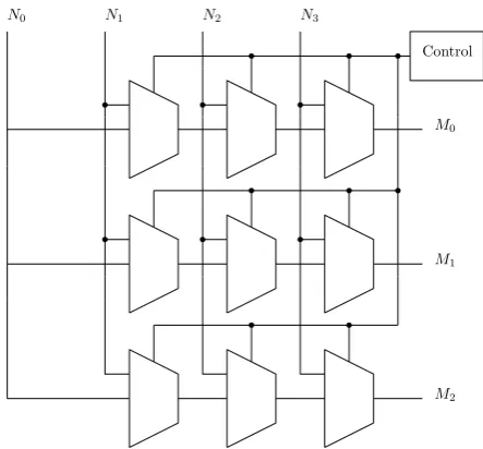
This Section describes the generation of the crossbar on hardware level. An architecture of anM rows byN columns crossBar is shown in Figure 8.2 forM =N = 3. The main property

is that every one of the inputsn⊆N can be directed tom⊆M. This can be accomplished

Automating system generation in Clash

Faculty of Electrical Engineering,

Mathematics & Computer Science

Automating System Generation

in C

λ

ash

Summary

List of acronyms

Contents

Chapter 1

Introduction

1.1 Problem description

1.2 Outline of this thesis

Part I

Chapter 2

C

λ

λ

λ

ash

2.1 Fundamentals

reg

i

f

o

s’

s

2.2 Higher Order Functions

f

xs!!0

f

xs!!1

f

xs!!2

a

b

2.3 REPL and simulation

2.4 Algebraic data types

Chapter 3

Comparison between existing SoC

communication standards

3.1 Characteristics of existing communication standards

3.2 Network on a chip

3.3 Comparison

Chapter 4

Existing Communication optimized

with C

λ

λ

λ

ash

4.1 Assignment of slaves to an address space

4

3

3

3

2

2

2

M

S

S

S

S

S

S

0x0

0xF

0x8

0xC

Addressing space

4.2 Communication with algebraic data types

Chapter 5

Hardware and data flow

5.1 Dataflow

v

Actor

Edge

Token

_f