Designing and visualizing a distribution network

DESIGNING AND VISUALIZING A

DISTRIBUTION NETWORK

ii

DESIGNING AND VISUALIZING A

DISTRIBUTION NETWORK

Bachelor Thesis Industrial Engineering and Management

September 20

_{, 2019}

Author

N. C. Meyknecht (Niklas) s1702505

Bachelor Industrial Engineering and Management

University of Twente Host Company

Drienerlolaan 5 Adres

7547 RW, Enschede City

Netherlands Country

First Supervisor Supervisor Host Company

Dr. P. C. Schuur (Peter) Name

Associate Professor Function

Dep. Of Industrial Engineering Host Company

and Business Information Systems Second Supervisor

Dr. D. Demirtas (Derya) Associate Professor

iv

P

REFACE

In front of you lies my bachelor thesis “Designing and Visualizing a Distribution Network”. This report

is part of my graduation assignment for my bachelor studies Industrial Engineering and Management. The research was performed at Company A in City A between April 2018 and September 2018 and consisted of researching the effects on the transport network following from an implementation of Company A’ distribution services in the French products network, in collaboration with Company B. I wish to thank Company A for having provided me with the opportunity of doing this research and expanding my skill set. I also wish to thank Supervisor Host Company for the continuous support at the office, but more importantly for the trust and autonomy. I also want to thank all colleagues in the office wing and Richard and Linda, my host family, for the enjoyable months.

Next, I want to thank Peter Schuur and Derya Demirtas for the quality and distinct feedback on my reports. Without their help, this report would not have achieved the condition is has now.

Finally, I want to thank my family and friends for the continuous support, which has driven me to reach for higher goals.

Have a nice read, Niklas Meyknecht

Enschede, September 2019

vi

M

ANAGEMENT

S

UMMARY

In this thesis I describe the bachelor’s assignment I have performed at the request of Company A, a logistical service provider in the European industry. The main service they provide is distribution of products all around Europe. They are partnered with local producers and large-scale retail organizations. One of these partners is Company B, a French garden center organization with around 200 retailers in France. They currently source their category A products through Company A services. Outdoor products are sourced at French producers.

At the time of the assignment, there was no comparable logistical service provider in France in the outdoor products industry, which Company A saw as an opportunity to expand their business. Company B, whose global market value of outdoor products currently is €70 million (€70M), is willing to make a commitment of products which Company B’s retailers would order through Company A. This commitment is defined as a fraction of the global market value, which is referred to simply as market value. Among other things, Company A needed to research how to organize transport around a new distribution center. Additionally, the results needed to be visually insightful to stakeholders, which include transport partners and producers, and the required market share should be high enough to be efficient but low enough as to mitigate the risks of the investment. This is the task I was set to do. The research question was prepared as follows:

How can the road transport network following from the implementation of Company A services in France be optimized, and how can results be visualized?

Optimization in this research is defined as the minimization of transport requirements of the network. As no system currently exists, the goal was to replicate the Dutch system in France with limited available data and knowledge and to observe the consequences and results from different scenarios. This research question can be more commonly described as a location-routing problem (LRP), an extension of the vehicle routing problem in which depot location and vehicle routing are included. Retailers order a number of carts, which are the transport trolleys in which products are stored for transport. When an order is passed, products are retrieved at producers, distributed in a distribution center (DC) and transported and delivered within three days between 08:00 and 12:00 or 14:00 and 18:00. The system should represent 52 weeks of deliveries with a single order each week. Through literature, we gained insights in the methodologies involved in a LRP: The objective function consists of four non-monetary measures: kilometers driven and trucks required to transport demand from DC to depots, and kilometers driven and trucks required to transport demand from depots and retailers. The transport between DC and depots and between depots and retailers are considered separately for the following reason: Transport between DC and depots are considered to transport exclusively Company A’ products, whereas transport between depots and retailers will be provided by the

transport partners. Their trucks could also transport products for unknown external retailers and are not necessarily assigned to one specific depot and do therefore not always return to originating depot. These measures are normalized, weighted and finally summed to score a given scenario, which we use as our cost function. Within this function we only seek to minimize transport requirements, not the minimization of transport costs. A set of 24 depots was made available by Company A’ French

vii

The LRP can also be defined as a Depot Allocation Problem (DAP) and a Vehicle Routing Problem (VRP), which we both approach using search procedures. With the planning horizon of 52 weeks, we have a chosen depot selection and market value which are fixed throughout the planning horizon. We do generate a transport network for every week using the following procedures, which are therefore repeated for every week of demand. Retailers are assigned to their nearest available depot as a starting solution for the DAP. This solution is improved upon with a TABU meta-heuristic. First, depot demand is determined by summing the total demand of a

depot’s assigned retailers. Each depot is supplied by n trucks

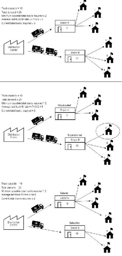
originating from the DC. We assume that the first n-1 trucks are filled fully, with the last truck transporting the remaining demand. We introduce the concept of depot saturation. The

saturation of depots determines the depot’s ability to accept

more retailer assignments, or its need to have retailers

unassigned to them. A depot’s last truck’s fill-rate determines the depot’s saturation: unsaturated,

saturated and supersaturated. If a depot’slast truck’s fill-rate is less than the average fill-rate of all last trucks, the depot it is due to is considered supersaturated: the depot’s last truck’s fill rate is low

to such an extent it is recommended to have retailers unassigned until the truck becomes obsolete. If the fill rate is more than average fill-rate of all last trucks, the depot is considered unsaturated: the

depot’s last truck’s fill rate is high enough that it is recommended to fill the truck to full capacity. If a

depot’s last truck’s fill-rate is 100%, the depot is considered saturated and it will not be selected to either have retailer unassigned from or reassigned to them. Additionally, its last truck’s fill-rate is not considered when determining the average last truck fill-rate. A random supersaturated depot is selected, and the retailer assigned to this supersaturated depot closest to another non-TABU unsaturated depot is selected and reassigned to this depot. This

origin depot is now TABU for this retailer for a given number of turns. A solution is accepted if a minimal number of trucks are required, which can be calculated using the known total demand divided by truck capacity, or if no improvement is measured for a given number of turns.

When the allocation process is complete, the VRP is approached. The procedure accounts for retailer delivery windows, truck carrying and driving capacities and the fact that trucks do not return at their originating depot. We do so by using an adapted maximum savings algorithm. First, the distance matrix between all locations is made asymmetric by setting all distances from retailers to depots to zero. Next, each retailer is assigned an exclusive route as a starting solution, in which this retailer is also the end point for the truck. For all possible connections between an origin and destination retailer, the expected savings are calculated by removing the increase in cost of the hypothetical connection from the total savings gained by removing an existing connection. This results in an asymmetrical savings matrix. By setting distances from

Figure 0-1: Example of the depot saturation method with an initial and final solution

viii retailers to depots to zero, the direction of a connection influences the savings as only one of the depot-retailer connections will be removed, as opposed to a depot-retailer connection for both retailers in the traditional Maximum-Savings method. The highest saving in the savings matrix is selected and temporarily implemented. The temporary route is checked for feasibility. A temporary

route’s current carrying amount and driving distance are updated. The delivery schedule of the route following from the new connection is updated by adding the destination route’s delivery schedule after the origin route’s delivery schedule, which we refer to as a push forward technique (the

destination route’s schedule is pushed forward). If no constraints are violated, the temporary

connection is implemented. If a connection is implemented, or if a connection is infeasible, the savings in the savings matrix are set to zero to prevent the connection from being selected again. In every route, the last retailer in the delivery schedule is also the end point for the route. The heuristic ends when the highest savings are zero or less. With this, routes are created every depot in every week. To implement the procedures, we required data concerning producers, depots and retailers. Available data was limited, and assumptions had to be made. It consisted of historical sales, transport and location records of a portion of Company B’s retailers for category A products procured via Company A’ services based in the Netherlands. Additionally, we obtained the production sizes of the 20 biggest producers and location information on the available depots. With the available data, we determined retailer specific demand pattern and developed a conversion method to convert euros to a cart count, which we use to convert a market value to a number of carts. Doing so, we can test different market values and obtain an associated demand. We also provided additional convincing to the decision of using City B as the location for the DC. Finally, real-road distances are gathered using a self-developed tool which gathers driving distances between locations as proposed by online mapping services. With the data and processes, we developed an analytical model which allows us to replicate a transport network for all 52 weeks of a scenario. In the model, the user can choose between testing scenarios with different market values and a fixed depot selection, of testing scenarios with different depot selections and a fixed market value. A scenario’s score is calculated using the previously defined KPIs. These KPIs are normalized, weighted and summed. This sum a scenario’s score: the lower the score, the better the scenario.

With this model, we tested the system for a range of market

values between €5M and €40M, five fixed depots selections and different KPI weights. This led to the conclusion that a

scenario’s efficiency increases as market value increases,

and that this increase in efficiency was unrelated to depot selections. We choose a market value of €20M as being a

starting value for further testing as after this market value the increase in efficiency slowed down considerably. Following this, we tested multiple depot selections with this fixed market value of €20M and multiple KPI weights. In order to provide faster results, we split the depots in four

geographical regions which we tested separately. For each region, the depots present in the more efficient scenarios were selected and tested on the global level. The 10 depots (including the DC, DEP6) can be seen in Figure 0-3. We tested against different weight combinations and market values of

€20M, €30M,€40M and€50M. Three depot combinations provided the most efficient results: - Combination 91, consisting of the DC and depots 4 and 22

- Combination 123, consisting of the DC and depots 4, 17 and 22 - Combination 223, consisting of the DC and depots 4, 17, 21 and 22

Figure 0-3: Depots present in the most efficient

ix

We notice that a combination of the four depots is most efficient each time. We compared the results visually for the different market values proposed and two different KPI weight sets: Set 1 has all KPIs equal with the KPI

“trucks required between depots and retailers” set to zero and Set 2 has all KPIs equal. With a market value of

€20M and KPI weight set 1, the most efficient depots

were depots DEP4 and DEP22. With a market value of

€30M or €40M, the most efficient depots were DEP4,

DEP17 and DEP22. With a market value of €50M, the

most efficient depots were DEP4, DEP17, DEP21 and

DEP22. With a market value of €20M or €30M and KPI

weight set 2, the most efficient depots were depots DEP4, DEP17 and DEP22. With a market value of €40M or €50M,

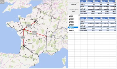
the most efficient depots were once again DEP4, DEP17, DEP21 and DEP22. In Figure 0-4, the visualization of a generated transport network can be seen. In this case,

this is the result of week 8 with a market value of €20M.

The active depots are the DC, depot 4 and depot 22. The visualization also shows the yearly and weekly fill-rates of the routes between the DC and depots. Following from these results, we recommend Company A to start by implementing their services with a market value of €20M and depots DEP4,

DEP6 and DEP22 with DEP6 functioning as the distribution center. As the market value and thus demand increases, DEP17 and finally DEP21 should also be used in the transport network.

1 Week 15 Week 16 Week 17 Week 18 Week 19 Week 20 Week 21 Week 22 DEP1 DEP2 DEP3 DEP4 DEP5 DEP6 DEP7 DEP8 DEP9 DEP10 94.5% 92.03% 92.97% 88.08% Year% Week% Year% Week%

Figure 0-4: Visualization of a generated transport network with recommend depots 4, 6 and 22

x

L

IST OF DEFINITIONS

Road Transport: All road-based transport driven by trucks

Global market value: The yearly turn-over for outdoor products for Company B

Market value: A share/commitment of the global market value, independent of geographical regions, product categories or suppliers.

Retailer market value: retailer specific share of the market value.

Depot demand: Sum of the demand off al retailers assigned to the depot

Last truck: The last truck n required to transport depot demand from DC to depot, carrying the remainder of demand the rest of which was transported by n-1 fully loaded trucks.

Average last truck fill-rate: average of the last truck fill rates of all depots, for the exception of depots considered saturated

Depot saturation: The depot saturation determines the depot’s ability to accept more retailer

assignments, or its need to have retailers unassigned to them.

Supersaturated depot: The depot’s last truck’s fill-rate is less than the average last truck fill-rates of all depots and therefore can have retailers unassigned from them

Unsaturated: The depot’s last truck’s fill-rate is more than the average last truck fill-rates of all depots and therefore can have retailers reassigned to them

Saturated: The depot’s last truck’s fill-rate is 100% and cannot have retailers unassigned from or reassigned to them.

Depot selection: Selection of depots for which a transport network is generated. Retailer: One of a customer’s businesses that sells the products

Customer: A large-scale retailer organization such as Company B

Category A products: Products intended for category A use, cultivated in Dutch producers Outdoor products: Products intended for outdoor use, cultivated in French producers

Season: Typical product selling season last during March, April and May. In this period, demand for products typically increases.

Carts: Transport trolleys, cc’s, in which products are transported in the products industry. Retailers must order enough products to fill carts to 95%.

Sequential method: A step by step method without feedback loops between de location problem solving and the routing problem solving

Iterative method: A looping step by step method with feedback loops between de location problem solving and the routing problem solving

Nested method: A method of solving the location problem by partially solving the routing problem

xii

L

IST OF

A

CRONYMS

• €##M: ## million euros

• LRP: Location-Routing Problem

• DAP: Depot Allocation Problem

• VRP: Vehicle Routing Problem

• MDVRP: Multi-Depot Vehicle Routing Problem

• VRPTW: Vehicle Routing Problem with Time Windows

• MDVRPTW: Multi-Depot Vehicle Routing Problem with Time Windows

• DC : Distribution Center

• DEP## : Depot number ##

• CDF: Cumulative Density Function

• KPI: Key Performance Indicator

• KM-In: Kilometers driven from DC to depots

• KM-Out: Kilometers driven from depots to retailers

• TR-In: Trucks required to drive from DC to depots

CONTENTS

Preface ... iv

Management Summary ... vi

List of definitions ... x

List of Acronyms ... xii

1 Introduction ... 1

1.1 Company A & Partners ... 1

1.2 Background assignment ... 2

1.3 Current situation ... 2

1.4 Problems and opportunities ... 3

1.5 Project Frankrijk ... 4

1.6 Deliverables ... 6

2 Theoretical framework ... 7

2.1 The Location-Routing Problem ... 7

2.1.1 Objective ... 7

2.1.2 Potential location & Present Sites ... 7

2.1.3 Search Procedure ... 8

2.1.4 Planning Horizon ... 8

2.2 Search procedures for the LRP ... 9

2.2.1 Exact methods ... 9

2.2.2 Heuristic methods ... 9

2.2.3 Meta-heuristics ... 10

2.3 Applications in literature ... 10

2.4 Choice of methods ... 11

2.5 Conclusions ... 12

3 Data analysis of the current transport network ... 13

3.1 Historical retailer demand and retailer geolocation ... 13

3.1.1 Global ordering distribution ... 13

3.1.2 Retailer demand ... 15

3.1.3 Cart value ... 16

3.1.4 Geolocation analysis ... 18

3.1.5 Additional characteristics ... 19

3.1.6 Conclusion Historical retailer demand and retailer geolocation ... 19

3.3 Depots ... 20

3.3.1 Distribution center ... 21

3.3.2 Conclusion ... 22

3.4 Transport ... 22

3.4.1 Transport characteristics ... 22

3.4.2 Distance matrix ... 23

3.5 Conclusion ... 23

4 Conceptual Model ... 25

4.1 Functioning of the analytical model ... 25

4.1.1 Objective function ... 26

4.2 Overarching component ... 27

4.3 Demand generation ... 27

4.4 Depot assignment ... 28

4.5 Vehicle Routing ... 29

4.6 Visualization ... 31

4.7 Conclusion ... 32

5 Experiments and results... 33

5.1 Experiment design ... 33

5.2 Assumptions ... 33

5.3 Market value ... 33

5.4 Depot selection ... 37

5.5 Conclusion ... 40

6 Conclusions and recommendations ... 41

6.1 Sub-questions... 41

6.2 Recommendations ... 43

6.3 Further research ... 43

Epilogue... 45

1

1

INTRODUCTION

In the finalization phase of my bachelor, Industrial Engineering and Management, I was offered the possibility of completing my study through an internship at Company A, researching the logistical consequences and effects following from an expansion opportunity. In this chapter, we introduce Company A and one of their key partners, Company B, and give some background on how Company A functions within their industry.

1.1

C

A

&

P

Company A is a logistical service provider in the European products industry. The main service they provide is distribution of products all around Europe. Daily, thousands of individual products travel across Company A’ distribution center (DC), located in City A, The Netherlands. They form the link between products producers, spread out over the Netherlands and neighboring countries, and retailer stores across Europe. The customer base is restricted to large-scale retailer organizations, such as IKEA and Praxis.

Company A was founded in 1882, and originally started as a products producer. In 2017, Company A traded near 100 million products to a total of 12 customers, generating 249 million euros in revenue. The second most profitable country was France, where two key customers of France are active: Truffaut and Company B. The latter plays an important role in this project.

Figure 1-1: Company A’ Distribution Center

2

represented €102 million (€102M) of revenue, consisting of €23M for category A-products, from which

€17M are provided by Company A, and €70M of outdoor-products.

1.2

B

As introduced, €17M of revenue in category A products is currently sourced through Company A, making Company A an important partner for Company B. €70M of revenue in outdoor products is currently sourced through many local (French) producers. These €70M are known as the global market value. On the 18th of April 2018, a meet-up was organized between different stakeholders in the French products industry, during which the prospects of an organized supply chain network for the outdoor products were discussed. Following this meet-up, Company A started “Project Name” with as

goal to implement their services in France. This assignment forms a part of this project.

1.3

C

Before engaging in the problem identification phase, the current situation in France and at Company A is summarized and some characteristics are defined. These characteristics apply to both situations. These consists of the transport carts, present in both networks, and the supply restrictions in the French and Company A network.

1.3.1 Carts

1.3.2 Category B-products France

The different retailers of Company B order their product individually. When ordering, they reflect on the different market trends, and determine which products to order. The retailers have to consider the restrictions put on by the producers. These restrictions can consist of product availability, minimum order sizes and costs. Producers organize their outbound transport themselves and will therefore only offer their own products except for occasional producer partnerships, which allow them to also offer partnered products. This, however, happens rarely. Exceptions to these operations are a few producers whose transport is being issued by Transport Partner B, a transport company who also runs a large portion of the current France-bound transport for Company A. These producers do offer organized transport.

1.3.3 Category A-products Company A

The processes at Company A can be summarized as an aggregated process of the above. Different producers inform Company A of their stocks for a specific period through the “Name”. Through

partnerships with the producers, Company A can offer products to their customers, consisting of the range of products each producer produces. Customers’ retailers can order carts, which they can fill with products of their choice for different producers. The most important restriction obliges retailers to fill their carts to an acceptable fill-rate (at least 95%). This is enabled trough an IT system, which inform retailers on the expected fill-rate of their to-order carts. Once orders have been received, products are collected at producers and transported to the DC at City A. For smaller producers, transport is organized by Company A or an external transporter. Larger producers organize transport themselves. Key to this process is that products from different retailers and different orders are transported to a central location. Once arrived, the distribution process starts, during which the products are distributed in new outbound carts according to the orders placed. After the distribution process, carts are loaded into trucks which will transport them to the retailers.

1.4

P

In this section, the problems and opportunities for improvement are described. They are categorized by the stakeholder directly involved in the issue.

1.4.1 Producers

Individual producers experience pressure from their customers: They wish ever so cheaper prices and lower ordering quantities. Producers, however, cannot provide their customers with the flexibility they expect. This leads to difficult customer relationships, and producers risk losing customers to competitors. Additionally, with the shrinking of order sizes and the difficulty to predict demand, producers are left with a higher workload.

Company A has identified several opportunities through an implementation of their services in France. First, by aggregating demand of several (smaller) stores through one ordering scheme, order sizes received by the producer will increase, full-time equivalents of products will be reduced and transport of products from producer to store would be improved. Additionally, there is an opportunity of implementing Company A’ services to automate the ordering process, resulting in less errors. Finally, Company A sees a lot of opportunities in a union between different producers.

1.4.2 Transporters

4

Opportunities observed by Company A are valuable options for an implantation of Company A in

France. Currently, there isn’t a transport service specialized in the products industry that provides transport nationwide. However, different transport partners, Transport Partner B and Transport Partner A, provide strong opportunities for nation-wide transport with the use of hubs spread over the country. Additionally, fill-rates of trucks has a lot of room for improvement. For instance, transport can be optimized by having products transported in one large batch by one party, instead of multiple parties having to make small deliveries (to potentially the same retailer). Transporters could also profit from a more stable prediction of transport needs and an optimization of transport routes.

1.4.3 Retailer (Company B Retail stores)

Most retailer problems and opportunities were elaborated on during the meeting on the 26th _{of April.}

Retailers experience problems with the minimum ordering sizes, especially for smaller retailers. The high minimum order size results in retailers having to order at least 3 carts of products from a producer. The variety of products a producer offers are limited to the partners of a producer, or the union they are part of (an aspect that is currently lacking in the French network.). This forces retailers to order too much of a certain type of product. This causes retailer to be left with a lot of overstock and prevents them from offering a higher variety of products in the same period, as this would result in even more overstocking. Another practical problem is that, when ordering from several producers, products arrive in an uncoordinated fashion. Additionally, they experienced a strong wish for cheaper products. On a higher management scale, Company B believes that they have too many suppliers. They have managed to reduce the number of producers they work with from approximatively 600 to approximatively 300, but this is far from their goal of being able to work with 20 producers, nationwide.

Opportunities Company A sees are, first, the solving of the experienced problems. They see a possibility of providing Company B retailers with orders consisting of products form several producers, with the number of products ordered from one specific producer by a specific retailer being less than a cart of products. By aggregating the products of several producers in the same carts, they can also solve the unconditioned transport issue. Finally, through economies of scale, they foresee a reduction in costs incurred on Retailers, something that is currently not in place. They also see opportunities of being able to select qualitative producers on a nation-wide scale and offer these products to the different retailers. They also noticed a lot of effort goes into the ordering process, mainly due to the required paperwork. With their services, they can digitalize this process, and eventually automate is, also resulting in less costs.

1.4.4 Company A

Company A is currently not active in the logistical network described. However, they do experience problems with it, as it conflicts with their norms and values. The transport network is highly unsustainable, both economically and environmentally. A second problem lies in the nature of the stakeholders. A lot of stakeholders from different background are involved in this network, some of whom are unfamiliar with Company A or lacking in understanding of how the processes work and why they are efficient.

1.5

P

N

1.5.1 Research definition

Relating the experienced problems and observed opportunities to the specific topic of this research, outbound transport, leads to a core problem: The outbound transport network is highly inefficient. With an implementation of Company A services in France, the organization of outbound transport can have a big effect on this efficiency of the transport network. The focus of this research is thus to optimize the transport network with an implementation of Company A services in France. With the wide variety of stakeholders involved in this project, the results should also be brought over in an insightful manner. This led to the following research question:

How can the road transport network following from the implementation of Company A services in France be optimized, and how can results be visualized?

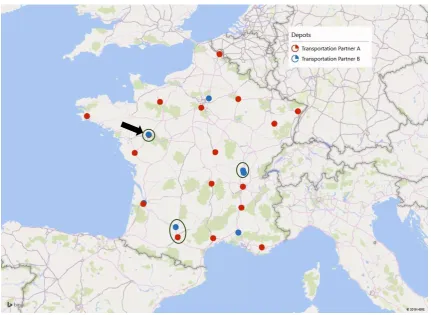
To do so, Company A has specified the specificities of the project. First, all inbound transport departing from producers will be directed towards a single DC, just as in their Dutch operations. We use the 20 most utilized producers by Company B, as the latter aim to reduce the number of different producers to such a number. Outbound transport from the DC to retailers can either directly be delivered at the retailers, or flow between depots. 24 depots are placed at our disposal by Company A’ French

transport partners: Transport Partner A and Transport Partner B. These are also the only transport partners we consider. All retailers must be supplied within three days of ordering. This lead time is generalised by using accepting a one-day lead time for all transport from producers to the DC as well as the preparatory distribution process overnight, a maximum one-day lead time for all transport between the DC and the depots and a maximum one-day lead time between the DC or depots and the retailers. A visualisation can be found in Appendix 7.7. Also, the DC location has been set to the region of City B (the relationship between the producers and the DC location and the conclusion to use City B are shown in Section 3.3). To answer the research question, we are required to deal with the multi-depot vehicle routing problem with time-windows (multi-multi-depot VRP with time-windows, or MDVRPTW), in which different scenarios are evaluated with each other. For each scenario, we analyze transport for 52 weeks (one year), with retailers ordering once a week. Within the VRP, an important requirement is that transport between two locations must be approximated with real geographical travel times and distances instead of straight lines. We elaborate on this in Section 3.4. Moreover, for transport between depots and retailers we assume transport will not exclusively consist of our products, and we therefor assume trucks do not return to depots after having delivered their products. Finally, Company A defines an efficient transport network as a network that satisfies their stakeholder satisfaction goals (e.g. delivery within three days of ordering) and contains minimum transport requirements. All results should also be visualized. To have products to transport, Company B must commit a number of products. This commitment is represented by a fraction of the global market value introduced in Section 1.2, which will be known as the (available) market value. The market value is not defined by certain product categories, certain geographical regions or even certain supplying producers. It rather influences the total ordering size of retailers in France.

Within the project we focus on the transport model in France, and therefor exclude all other countries. We also have limitations with the available data and will therefore make use of assumptions. Finally, this project serves to give a strategic advice and will there not consist of the implementations and evaluations of the project.

1.5.2 Plan of approach

6

a clear majority of options will form an optimization. The enveloping plan of approach is to build a What-If analysis to assess which scenarios are most efficient.

To answer the research question, several sub-questions must be answered, related to the different aspects that play a role in this transport network and its optimization and visualization. For these sub-questions, data and information is gathered through literature research, (semi-)formal interviews with stakeholders, available datasets and data generation in the case of missing data.

1. Which insights can literature give us on solving comparable problems? 1.1. What are the methodologies in similar problems?

1.2. What theories exist to solve these problems? 1.3. What methods have been applied in the past? 1.4. What is our choice of methods?

Through a literature review, we analyze which methodologies apply to our situation. We first research the methodologies that apply and common theories in which routing network problems are commonly addressed. Second, we analyze past research to discover how routing problems were solved and how we can use these to answer our research question. Finally, we define the method we use in the project. 2. How is the French transport network organized?

2.1. What are the characteristics of Company B Retailers? 2.2. What are the characteristics of depots?

2.3. What are the characteristics of transport?

The research question aims to define how the network is currently organized. The limited data available is processed to obtain insightful data on ordering habits, depot and DC locations and transport characteristics. Additionally, it determines how we can convert a market value to a cart demand.

3. How is the transport network influences by a varying market value and depot selection?

3.1. What is an adequate market value for initial testing?

3.2. Which depots contribute most to a more efficient network?

3.3. How does the market value influence the more efficient depots?

The research question aims to determine how the network efficiency varies under altering conditions. First, we research the effect of the market value on the network efficiency with arbitrary example networks to determine which market value we should use as a begin point to satisfy Company B’s

need for a low market as well as to provide a network whose efficiency is satisfying enough. Second, we research which depots provide the most efficient depot under this market value. These depots are finally tested against varying market value to also analyze the effect of an altering market value on the choice of efficient depots.

4. Conclusion and recommendations

From the previous research questions we can draw conclusions and answer the key research question. We also offer our recommendations to Company A, consisting of depot combinations to use at different market values.

1.6

D

7

2

THEORETICAL FRAMEWORK

In this section, we explore the literature on depot implementation strategies. In Operations Research, this is also known as the Location Routing Problem (LRP), consisting of a Location/Depot Allocation Problem (DAP) and a Multi-Depot Vehicle Routing Problem (MDVRP). In Section 2.1, we explore the methodologies involved. In Section 2.2, we expand on the different search procedures that apply in an LRP. In Section 2.3, we review past application of LRP solving methods. In Section 2.4, we define our LRP and we develop the methods we use to approach the LRP.

2.1

T

L

-R

P

According to Tai-Hsi Wu (1999), the LRP is defined to find the optimal number and locations of the depots, simultaneously with the depot allocation, vehicle schedules and distribution routes so as to minimize the total system costs. Francis & Goldstein (1973) published a list of 216 references, which was later complemented by Rand (1976). The latter argues that seven choices need to be made when determining the procedures to be adopted in a depot location study. We will focus on five: the objective, the potential locations, the present sites, the search procedure and the planning horizon.

2.1.1 Objective

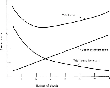
The objective has typically been to minimize costs, and it often thought that this is reached through a lowest number of depots. On an economical scale, the costs resulting from depots largely depends on the fashion in which depots function together. In his report, Beattie (1973) found different variable costs determine the total cost of a depot, considering only transport and depot costs. It is more important to have depots in the right place, than to have the right number (Beattie, 1973).

In addition, Mercer (1970) adds that as the distance from a depot increases, the market share declines with the presence of large number of competitor or a well-defined competition.

These examples show that an objective function should be chosen taking in account all relevant factors to the situation. Examples of objectives include customer relationship by allowing decreased delivery time and therefore allowing them to carry a lower inventory, or the return of investments following from a larger market share due to a lower customer distance.

2.1.2 Potential location & Present Sites

When approaching a LRP, the depot location possibilities must be defined. Revelle, Marks, & Liebman (1970) provide the researcher with two approaches: All points on a plane, or points on the network. When considering all point on a plane, an infinity of options is available each characterized by some form of distance measurement to the nodes (i.e. retailers). When considering points on a network, a

Figure 2-1: Annual cost vs number of depots (Beattie, 1973)

8

finite amount of locations is known before-hand, in which all options are also characterized by some form of distance and time measurement. These two options are also called an infinite of a feasible location set, which can be compared to a continious or discrete location set. When using a feasible location set, present known sites can be used as the location set. Revelle, Marks, & Liebman (1970) collected different researches and summarized their depot location strategies. Methods all revolve around an objective function (as discussed above) in which the goal mostly is to minimize transport and location costs. Additionally, the capacities of the depots can be considered, defining the difference between capacitated and uncapacitated LRPs.

Mercer (1970) acknowledges both methods, but also gives critic to both. The infinite set approach cannot guarantee a (near) optimal solution but merely a best solution for a given starting point. Also, found solutions can be infeasible when applied in practice, due to region specificities or laws and regulations. Finally, no method exists to determine the optimal number of depots. The finite set approach is criticized by its limitation to find an optimal solution. To do so, many locations are required. An additional consideration when using a finite number of locations approach is to use present known sites, for instance when considering a merger between two companies.

2.1.3 Search Procedure

Along with the choice between an infinite or finite set approach is the choice of search procedure. The search procedure dictates in which fashion the LRP will be tackled. Mercer (1970) shows four methods; simulation, heuristics, integer programming with feasible set and the infinite set approach; are classified based on the complexity of the cost function, of objective function, and the search procedure for finding depots.

The choice of search procedure is applicable to many VRPs. Common methods are exact methods, heuristics, metaheuristics and simulation studies. Exact methods allow the finding of optimal solutions through an algorithmic approach but are very time-consuming in real-world situations. Heuristics have been developed to shorten the processing time by continuously improving a given or random starting solution, however they do not necessarily give an (near) optimal solution and can get trapped in a local optimum. Meta-heuristics are procedures designed to find a heuristic to find solutions for optimization problems. They have a larger search space than typical heuristics and can temporarily accept deteriorating solutions, preventing them being stopped at a poor level local optimum. Finally, simulation is a solving method. In a simulation the conditions of a real-world

system are replicated. Optimization occurs by analysing the stochastic influences on given solutions and deciding on the most efficients ones. Search procedures will be further researched in Section 2.2

2.1.4 Planning Horizon

Some researchers claim that depot locations are strategic problems, as opposed to VRPs which are tactical problems because routes can be redefined frequently, whereas depot locations are usually for

Figure 2-3: The relationship between complexity in search procedures and cost functions. (Mercer, 1970)

longer periods of time, and thus over a longer planning horizon. The same planning framework was there for inadequate (Nagy & Salhi, 2006). These claims were revoked after investigations proved that the use of a location-routing framework would reduce costs over long planning horizons (Salhi & Nagy, 1999). Therefore, a framework should be defined by the researcher. It was also advised to use a long planning horizon as opposed to a static situation.

2.2

S

LRP

The LRP and the MDVRP are spin-offs of the VRP, a well-known and researched challenge in the operations research. The LRP is defined as the process where the optimal number, the capacity, and the location of facilities are determined, and the optimal set of vehicle routes from each facility is also sought (Marinakis, 2009). The MDVRP focusses on the assignment of retailers to depots based on an available set of depots and the ensued routing of vehicles. As described in Section 2.1, the LRP and MDVRP require an objective function, a choice of approach between infinite and finite depot sets, a planning horizon and search procedures. In this section, we will address search procedures applied in previous research which tackled LRPs and MDVRPs.

2.2.1 Exact methods

Exact methods are methods which guarantee an optimal solution to a given problem. Due to their computation time, these methods are usually only applied on small theoretical problems. Cooper L. (1961) proposed a method where the location of m number of depots were optimally placed on a plane surface by finding the point which minimized the Euclidian distance between the destinations and the different depots, as one of the first solutions to the location problem defined by Alfred Weber in 1909 (Revelle, Marks, & Liebman, 1970). Nagy & Salhi (2006) summarized several different methods applied by previous researchers.

2.2.2 Heuristic methods

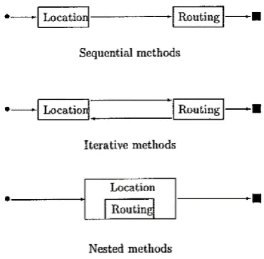
When applying heuristics to a LRP, the problem becomes twofold: a locational problem and a routing problem. Salhi & Nagy (1999) described three methods within which heuristics can be classified: sequential, iterative and nested methods.

Sequential methods process the LRP by first locating the depots and secondly by approaching the routing problem. In this method, there is no feedback loop. Iterative methods combat this problem by following a loop in which the output for each sub problem is used as feedback for the other sub problem to be tackle more efficiently. Nested methods view the location problem as key, with the routing problem being referred to in a subroutine. The routing problem

generally isn’t fully solved, and estimations are used to serve as feedback for the location problem.

Lim & Wang (2005) showed two methods, a two-stage and a one-stage method, which tackled the MDVRP. These methods are comparable to the sequential and the nested methods, showing the methods apply for MDVRP heuristics as well.

10

2.2.3 Meta-heuristics

Heuristics are mostly problem dependent, meaning they are developed to fit a very specific problem. Meta-heuristics are problem independent techniques. Osman & Laporte (1996) define it as an iterative generation process which guides a subordinate heuristic. Meta-heuristics can be classified, among others, in the following categories:

- Local and global search: as defined in Section 2.1.3, this determines whether the meta-heuristics aims to reach a local or a global optimum. Global search meta-meta-heuristics use probabilistic methods to allow a deterioration of the current optimal solution.

- Single and population-based solutions: They define the size of the solution set from which the meta-heuristics’ iterations improve on. A single-solution-based solution set means that a single solution is altered and selected. A population-based solution set means the meta-heuristic determines an ideal solution from multiple possible solutions.

Common meta-heuristics are applied a variety of fields, including operations research. A common meta-heuristic is TABU. This method generates a neighborhood of solutions from a starting solution using different iterations. Within this neighborhood, the best scoring solution is implemented. This solution does not necessarily have to be an improvement on the initial solution. When a iteration is implemented, this iteration is considered forbidden, or TABU, for a number of iterations. This process repeat until an ending criterion has been met, after which the best scoring solution over all iterations is implemented. Simulated Annealing also explore a neighborhood, but selects a solution based on a randomness factor. From a neighborhood, a single solution is selected. Through a cooling factor, a probabilistic function determines whether this solution is accepted or not. This function is influenced by the observed improvement or deterioration, and the number of steps already taken. Genetic algorithms translate multiple solution into a genetic code, which are combined to create a new genetic code. This is done by selecting how the origin codes interact with each other to combine their genomes in one child genetic code.

2.3

A

(2002) present a sequential metaheuristic optimizing the LRP by considering the problem as a DAP and a VRP, considering depot capacities. Both problems are solved using tour and retailer swaps or insertions respectively. To improve results, the DAP follows a SA framework and the VRP follows a combination of both TABU and SA. Renaud, Boctor, & Laporte (1996) describe a TABU meta-heuristic involving a three-step method, FIND. In the last two steps, the solution neighborhood consists a single vertex being altered. The latter is TABU whenever that depot it is assigned to changes. The meta-heuristics neighborhood thus consists of a single solution (Section 2.2.3) as opposed to many proposed TABU implementations.

2.4

C

Most of the sources use an objective based of fixed and variable costs for depots usage and vehicle usage. Others focus on different aspects of the transport network such as the minimization of truck idle time or the number of trucks used. The optimization goal, as defined by Company A, is to provide efficient transport. Our objective will therefore consist of the minimization of kilometers driven by trucks, and the minimization of truck usage. We leave depot usage costs out of the studies as our objective is to provide minimum non-monetary transport requirements which are not influenced by depots costs. We consider delivery time as a hard constraint. We also use a selection of 24 present sites as a depot location set. Our planning horizon is a year of 52 time-instances (weeks). The search-procedure follows a sequential method. At first, retailers are allocated to available depots. The depot selection is fixed for all 52 instances, however depot-retailer allocation and vehicle routes will be recalculated each instance.

For each week, an initial DAP-solution will be created by assigning all retailers to their nearest depot. The DAP-solution is improved via a TABU meta-heuristic. First, the total demand of all retailers assigned to a depot is determined for each depot, called the depot demand. Second, as depots are supplied by the DC, n trucks are required to transport the depot demand to the depots. We assume that n-1 trucks are filled to maximum capacity, with the last truck transporting the remaining demand. This truck’s fill-rate is called the last truck’s fill rate. We introduce the concept of depot saturation. Saturation of depots determines the depot’s ability to accept more retailer assignments, or its need

to have retailers unassigned to them. A depot’s last truck’s fill-rate determines the depot’s saturation:

unsaturated, saturated and supersaturated. If a depot’slast truck’s fill-rate is less than the average fill-rate of all last trucks, the depot it is due to is considered supersaturated: the depot’s lasttruck’s

fill rate is low to such an extent it is recommended to have retailers unassigned until the truck becomes obsolete. If the fill rate is more than average fill-rate of all last trucks, the depot is considered unsaturated: the depot’s last truck’s fill rate is high enough that it is recommended to fill the trucks to full capacity. Finally, depots can become saturated: if a depot’s last truck’s fill rate is 100%, the depot’s

retailer allocation is considered optimized and will therefore not be selected for either having a retailer unassigned from or reassigned to them and its last truck’s fill rate will not be considered when

determining the average last truck fill-rate. Next, a random supersaturated depot is selected. One of the retailers assigned to this depot will be reassigned to an unsaturated depot. Of all the

supersaturated depot’s assigned retailers, the retailer closest to a non-TABU unsaturated depot will be reassigned to this depot. This iteration is now TABU for a given number of iterations. This process is repeated until a minimum number of trucks required to transport all demand to all depots is reached, or until no improvements have been observed for a given number of turns. The minimum number of trucks required can be calculated by dividing total demand by truck capacity. With the search-procedure, we tactically aim to reduce the required amount of trucks: the supersaturated

12

reduce the last truck’s fill-rate until it becomes obsolete. For the unsaturated depot’s last truck, we

aim to increase its fill-rate until it reaches maximum capacity.

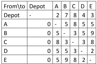
When the allocation process is complete, the VRP is approached. The solving procedure accounts for retailer delivery windows, truck carrying and driving capacities and the fact that trucks do not return at their originating depot. We do so by using an adapted maximum savings algorithm. First, the distance matrix between all locations is made asymmetric by setting all distances from retailers to depots to zero, which enables trucks to not return to depots and end at the final retailers. Next, each retailer is assigned an exclusive route as a starting solution, in which this retailer is also the end point for the truck. For all possible connections between an origin and destination retailer, the expected savings are calculated by removing the increase in cost of the hypothetical connection from the total savings gained by removing an existing connection. This results in an asymmetrical savings matrix. By setting distances from retailers to depots to zero, the direction of a connection also influences the savings as only one of the depot-retailer connections will be removed, as opposed to the removal of the depot-retailer connection for both retailers in the traditional Maximum-Savings method. The highest saving in the maximum savings matrix is selected and temporarily implemented. The temporary route is checked for feasibility, it’s current carrying amount and driving distance are updated and the delivery schedule of the route following from the new connection is updated by

adding the destination route’s delivery schedule after the origin route’s delivery schedule, which we

refer to as a push forward technique (the destination route’s schedule is pushed forward). If no

constraints are violated, the temporary connection is implemented. If a connection is implemented, or if a connection is infeasible, the savings in the savings matrix are set to zero to prevent the connection from being selected again. In every route, the last retailer in the delivery schedule is also the end point for the route. The heuristic ends when the highest savings are zero or less. With this procedure, routes are created every depot.

2.5

C

13

3

DATA ANALYSIS OF THE CURRENT TRANSPORT NETWORK

This chapter consists of the data collecting process. We collect data from databases, (semi-formal) interviews and internet, and we process the data to make it workable. In Section 3.1, we analyze retailer information to obtain retailer locations, sizes and demand patterns and we develop a method which converts a market value to a number of carts ordered. In Section 3.2, we show insights in producer supply. In Section 3.3 we present the available depots and their locations and substantiate Company A’ call to use depot 6 (DEP6) as a DC. In Section 3.4, we define the transport constraints and obtain a real-road driving distance matrix between all available locations.

3.1

H

To estimate future demand, a historical analysis is required. The historical analysis of demand for outdoor products of the Company B retailers in the French network is hard to obtain: Company A has only been involved in the supply of category A products sourced from the Netherlands. Additionally, Company B is unwilling of sharing their data with us. We must therefore find another way of estimating the demand history of Company B retailers using data we can obtain. We have chosen to use the transaction history of all products sourced by Company B through Company A. This data set contains information about different Company B retailer that can allow us to analyze historical demand. By doing so, we make two assumptions:

Assumption 1: Retailer ordering history of category A products sourced through Company A is an accurate representation of the retailer ordering history of category B products sourced through local producers

Assumption 2: Retailers ordering through Company A represent the totality of Company B retailers in France.

Assumptions allow progress in the progress and prevent cutbacks in the reliability and feasibility of the project, as historical data is essential. This is the most accurate data source available to Company A. Also, not all Company B retailers order through Company A, resulting in assumption 2.

We have three datasets at our disposition for the analysis: the transaction dataset the transport dataset and the producer dataset. The transaction dataset contains the transaction history of all Company B retailers. It’s a spreadsheet of transactions, containing time and customer information, order information such as products ordered, the price and expected fill-rates of the carts. This last measurement is used while ordering to ensure that an order is, ideally, always optimally filled as introduced in Section 1.3.3. This dataset also provides information on the value of carts. The transport dataset contains historical information concerning carts recorded after the distribution process as they are loaded in trucks to be transported to the retailers. It contains information about the loading date, expected delivery date, customer information and the number of carts to be transported. This dataset provides more factual information of the number of carts transported following from an order. From this dataset we also obtained location information of retailers. The producer dataset was provided by Company B and contained monthly supply information of their top 20 producers.

3.1.1 Global ordering distribution

14

separates all three years to identify particularities that apply to only a specific year, whereas Table 3-2 aggregates this information into one year.

Table 3-1 Weekly global demand between 01/01/2016 and 05/06/2018. Product turnover refers to the relative demand in carts in weeks within that year.

Table 3-2 Weekly global demand with yearly data combined between 01/01/2016 and 05/06/2018.

We can notice two trends: sudden peaks and seasonal demand. Sudden peaks are caused by discount periods, which can apply to some or all retailers. The peaks in week 3 of 2016 and 6 & 8 of 2018 are explained sporadic discount periods. Peaks in week 33 and 34 of 2016 and 2017 are caused by the Rentrée discount period, popular in France when the school year starts. In week 48 of 2017, a Christmas discount is observed. The remaining change of ordering volume follows from seasonality. Seasonality of demand is present in the whole flower industry. Practically all retailers Company A provides to follow a comparable seasonal pattern. The months March, April and May are considered

“on-season”. The ordering volume increases significantly during this period. Week 8 to 22 represent an average of 2.66% ordering volume, compared to average of 1.62% outside these bounds, including discount periods.

Ideally, we wish to identify seasonality and discount demand separately, to accurately estimate order volume in a prediction model. However, no distinction can be made between these orders. We therefore cannot separate discount orders from regular order. We assume that the occasional discount orders belong to the regular demand. As a side-note, the Rentrée and Christmas discounts have a significant probability of occurring in the future as well and are therefore important to consider.

Assumption 3: Discount orders belong to regular demand.

0,00% 1,00% 2,00% 3,00% 4,00% 5,00% 6,00% 7,00% 8,00%

1 3 5 7 9 11 13 15 17 19 21 23 25 27 29 31 33 35 37 39 41 43 45 47 49 51

Pro d u ct tu rn o ve r Week

Weekly global demand (years separated)

2016 2017 2018 0,00% 1,00% 2,00% 3,00% 4,00% 5,00% 6,00%

1 3 5 7 9 11 13 15 17 19 21 23 25 27 29 31 33 35 37 39 41 43 45 47 49 51

Pro d u ct tu rn o ve r Week

3.1.2 Retailer demand

In this section, we analyze the different retailer sizes and elaborate on some specific cases. Doing so, we wish to develop insight in the variety of retailers present in the French network to substantiate possible future decision that will have to be made. The following histogram shows the number of times retailers have ordered.

Table 3-3 Retailer sizes based on the amount of times ordered. On the horizontal axis, the number of times ordered over the period are indicated, with the count of their recurrence on the vertical axis.

The average number of times ordered is 93.3. Over 131 weeks of data, retailers order every 0.71 weeks on average, or approximately twice over three weeks. The variance is also high. Retailers follow an individual ordering schedule. In the following chart, all retailer ordering sizes relative to the retailers total ordering size are compared to determine whether differences in ordering size and ordering frequency result in a difference in demand patterns. If not, we could suggest using a universal demand pattern for all retailers.

Table 3-4 Weekly ordering size per retailer. The 52 weeks in a season are represented on the horizontal axis. The retailers are represented on the vertical axis. The ordering size is represented on the z-axis, shown in colors.

0 10 20 30

2 14 27 39 52 64 76 89 101 113 126 138 151 163 175 188 200

Re

cu

rre

n

ce

Order count

16

We performed as statistical test to determine whether all retailers follow the same global ordering trend. Our hypothesis, h0, is that all retailers follow the same distribution. The average week specific ordering size over all retailers are determined and used as a global relative ordering size per week, which would apply for all retailers.

A popular statistical test is the Chi-squared test. However, the occasional order counts of 0 prevent the usage of this test. Our data also consists of more than 20% of orders less than five. Also, we expect retailers to occasionally order 0 products. A relatively unknown statistical significance test is the G-test, a replacement for the Chi-squared. It is more fit for our data and we have therefore opted to use it. The following functions and restrictions apply to both the Chi-squared and the G-test:

G-test 𝐺 = 2 ∗ ∑ 𝑂𝑖∗ ln(

𝑂𝑖 𝐸𝑖 ) 𝑖

𝑂𝑖 ≥ 0 𝑓𝑜𝑟 𝑎𝑙𝑙 𝑖 𝐸𝑖 > 0 𝑓𝑜𝑟 𝑎𝑙𝑙 𝑖

Chi-Squared test

𝜒2= ∑(𝑂𝑖− 𝐸𝑖) 2

𝑂𝑖 𝑖

𝑂𝑖 ≥ 5 𝑓𝑜𝑟 𝑎𝑡 𝑙𝑒𝑎𝑠𝑡 80% 𝑜𝑓 𝑖 𝐸𝑖 ≥ 1 𝑓𝑜𝑟 𝑎𝑙𝑙 𝑖

Using a 95% significance, we concluded that we must reject our hypothesis. Thus, retailers do not follow the determined distribution pattern. We performed an additional test using a weighted distribution in which high ordering retailers have more influence on the distribution, which also resulted in the hypothesis being rejected. We conclude from this that the retailers do not follow a global ordering trend. All must be assessed individually. The statistical hypothesis tests can be found in Appendix 7.3

3.1.3 Cart value

Table 3-5 Histogram of fractions of carts purchasable with one euro

The high deviation in cart values led to the decision to use a distribution for the cart value, instead of using an average. Using an average cart value leads to an unvarying retailer demand when implemented in the analysis. Testing a same depot selection and market value multiple times would lead to identical results. Using EasyFit, the fitting distribution found is a three-parameter log-logistic with the parameters given below. We reversed the Cumulative Density Function (CDF) to retrieve a specific cart value based on a random variable:

𝐶𝑎𝑟𝑡 𝑣𝑎𝑙𝑢𝑒 = 𝛽 ∗ (( 1

𝑟𝑎𝑛𝑑) − 1) −1_𝛼

+ 𝜆

𝑟𝑎𝑛𝑑 = [0,1]

𝛼 = 4.6834 𝛽 = 0.00070558 𝜆 = 0.00074104

This distribution fits only given the market values observed in the data. Cart values can vary as demand increases or decreases. We assume the function is reliable and accurate for a changing market value.

Assumption 4: The cart value function is reliable and accurate.

Finally, the value of carts for outdoor products in the French industry is less than the value of carts for category A products at Company A. The transport team at Company A estimates that for a given value a retailer can order twice as much outdoor products carts. This means retailers can buy twice as high fraction of a cart with one euro. We therefore multiply the resulting cart value by two.

Assumption 5: The value of outdoor-products carts is half the value of category A-products carts.

The conversion is done after the global market value has been distributed over all retailers and weeks to provide every retailer with an arbitrary cart value every week, to approach a scenario in which carts have different values. Thus, retailers with identical order value might order different numbers of carts. We end with the following function calculating the carts ordered based on a given budget.

0 100 200 300 400 500 600 700 800 900 0.0 81% 0.0 89% 0.0 97% 0.1 05% 0.1 13% 0.1 21% 0.1 29% 0.1 37% 0.1 45% 0.1 53% 0.1 61% 0.1 69% 0.1 77% 0.1 85% 0.1 93% 0.2 01 % 0.2 09% 0.2 17% 0.2 25% 0.2 33% 0.2 41% 0.2 49% 0.2 57% 0.2 65% 0.2 73% 0.2 81% 0.2 89% 0.2 97% 0.3 05% 0.3 13% 0.3 21 % Mo re Fr e q u e n cy

Bin (percentage of a cart)

0,001 0,0015 0,002 0,0025 0,003

0,01 0,08 0,15 0,22 0,29 0,36 0,43 0,50 0,57 0,64 0,71 0,78 0,85 0,92 0,99

Cart

valu

e

Probability

18

𝐶𝑎𝑟𝑡𝑠 = 𝑟𝑜𝑢𝑛𝑑 (𝑀𝑉 ∗ 𝐶𝑆 ∗ 2 ∗ (𝛽 ∗ (( 1

𝑟𝑎𝑛𝑑) − 1) −1_𝛼

+ 𝜆))

𝑀𝑉 = 𝐺𝑙𝑜𝑏𝑎𝑙 𝑀𝑎𝑟𝑘𝑒𝑡 𝑉𝑎𝑙𝑢𝑒

𝐶𝑆 = 𝐶𝑢𝑠𝑡𝑜𝑚𝑒𝑟 𝑆ℎ𝑎𝑟𝑒

3.1.4 Geolocation analysis

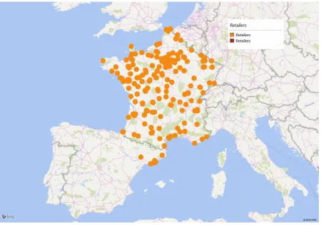
Using a tool available in Excel, 3D Maps, we link the findings in Section 3.1 so far to coordinates on a map. GIS locations are provided in the transport dataset. This section focusses on showing how the data is spread over France. In the figure below, all available retailers are depicted on a map.

Figure 3-1: Retailer locations

Some retailers are in Spain and in Portugal. The scope defined in Section 1.5.2 cites we include only the French and eastern Spanish retailers. From a strategical point of view, we argued that as the eastern Spanish retailers are relatively close to France, we can include them in our research. The other foreign retailers are too far to include in the network. We therefor assume the eastern Spanish retailers are included in the French transport network.

Assumption 6: Eastern Spanish retailers are included in the French transport network.

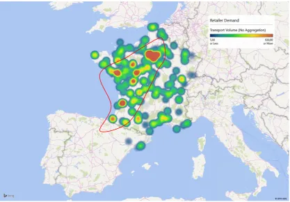
Figure 3-2: Retailer demand. The highest demand area is encircled in red.

3.1.5 Additional characteristics

Through semi-formal interviews with the Company A Transport team, we know retailers can only accept deliveries during their opening hours, which are between 08:00 and 12:00, and between 14:00 and 18:00. Some retailers only accept deliveries during one of these timeslots, but the Transport team sees a growing trend of retailers receiving deliveries during both time slots. We therefore assume that all retailers can be delivered to during both time slots.

Assumption 7: Retailers can be delivered at between 08:00 and 12:00, and between 14:00 and 18:00.

Additionally, we have assumed the ordering frequency of depots. As we do not have exact data, we have limited our research by assuming retailers order only once a week, thus 52 times a year.1

Assumption 8: Retailers order once a week at most.

3.1.6 Conclusion Historical retailer demand and retailer geolocation

In this sub-section, we analyzed available on retailers. Due to restrictions described in Section 1.9, we made some assumptions concerning the reliability of our data. Nevertheless, we conclude that due to a considerable difference in retailer sizes and ordering patterns, all retailers should be assessed individually when estimating their demand. This leads to the usage of empirical ordering data in the future. Additionally, we charted the different retailers (and their demand) on a map from which we concluded that including the eastern Spanish retailers to our scope is a good strategical decision. We also concluded that retailers can be delivered at during time-slots applicable to all retailers, that

1 _{Later during the project, on the Date, Company B’s Sales Manager explained he expects his retailers to order}

twice or thrice a week, due to the freedom of restrictions (e.g. minimum 3 carts per nursery) offered by