Munich Personal RePEc Archive
On development paths minimizing the
structural change costs in the
three-sector framework and an
application to structural policy
Stijepic, Denis
University of Hagen
14 February 2017
1
On Development Paths Minimizing the Structural Change Costs in the Three-Sector
Framework and an Application to Structural Policy
Denis Stijepic*
University of Hagen
14th February 2017
Abstract. Structural change is associated with high costs for the economy and the society
ranging from environmental pollution to unemployment. We focus on the three-sector
framework (related to agriculture, manufacturing and services) and assume that the structural
change costs increase with the strength of structural change. We show that monotonous
structural change paths are minimizing the structural change costs in this framework. By using
this result and the (qualitative) stylized facts of structural change based on the theoretical and
empirical literature consensus, we derive the cost-minimizing strategy for a developing
country. We use these results to discuss some well-known structural/trade strategies.
Keywords: employment, structure, transformation, industrial, structural, policy, costs, long
run, geometry, vector, simplex, dynamic optimization, uncertainty, calculus of variations.
JEL: O14, O41, O21, O24, C61
_________________________________
*Address: Fernuniversität in Hagen, Universitätsstrasse 41, D-58084 Hagen, Germany. Phone: +4923319872640.
2 1. Introduction
1.1 Motivation of the Paper
One of the key characteristics of the long-run development process is structural change as
measured by the long-run changes in the sectoral GDP and employment shares. We focus on
the three-sector framework dividing the economy into the agricultural, manufacturing and
services sector, which has been studied in numerous empirical and theoretical studies.1
Structural policy within the three-sector framework means fostering policies (e.g., choosing
taxes, tariffs, subsidies, education system structure, infrastructure, research funding schemes
and legal entry barriers) that favor one sector over the others. The development literature
provides different arguments for such structural policy, as discussed in Section 2. Some of
these arguments are favoring agriculture, while others are favoring manufacturing or services.
Moreover, as shown in Section 2, most of the arguments (a) refer to an underdeveloped (i.e.
not fully industrialized country) that seeks for an optimal structural policy (in the three-sector
framework) over the initial phase of its development and (b) do not address the myopic
development planer or policy maker (who seeks to maximize initial growth, while neglecting
the long-run effects of its policy), but the planer who seeks to maximize and sustain the welfare
and growth in the long run; i.e. the arguments refer to the effects of the present-day’s policy in
a more or less distant future.
Our paper is a contribution to this discussion of optimal structural policy in the three-sector
framework. We focus on the costs of structural change; in particular, we assume that the
economic and social costs of structural change increase (monotonously) with the magnitude of
structural change (as measured by the magnitude of the changes in the sectoral employment
shares or sectoral GDP shares). The historical experiences of present-day’s developed and
developing countries reveal severe costs of structural change, among others, increasing
environmental pollution and global warming (over the industrialization phase), costs associated
with unemployment (over the de-industrialization phase) and geographical re-location of labor
(e.g. negative aspects of hasted urbanization over the industrialization phase) and
abandoned/unused/sunk capital, e.g. ghost cities/facilities (over the de-industrialization phase).
These costs are still being discussed in highly developed economies (e.g. in election
campaigns), which reveals their lasting impact on the society.
1 For an overview of the structural change literature, see, e.g., Schettkat and Yocarini (2006), Krüger (2008), Silva
3 1.2 Aims of the Paper
Considering the magnitude of the structural change costs, it seems to make sense to discuss the
structural policy alternatives based on the structural change costs they cause. In particular,
following the discussion from above (cf. points (a) and (b)), we search for an answer to the
following (theoretical) problem: assume that the non-myopic (cf. point (a)) social planer in an
underdeveloped (i.e. non-industrialized) country seeks to choose a structural policy over the
initial development phase of its country that minimizes the future structural change costs (over
the planning horizon); which structural change path (among the many feasible structural
change paths) should the social planer choose? We provide a solution to this
calculus-of-variations problem and demonstrate that it can be used to (i) design a structural policy that
minimizes the structural change costs in a developing country, (ii) evaluate the prominent
structural policy alternatives discussed in the literature based on the structural change costs
they cause and (iii) easily estimate the aggregate magnitude of the past structural change costs
beared by the present-day’s developed economies on the basis of macroeconomic historical
data (cross-country comparison of cost-efficient structural change).
1.3 Method/Approach
We model structural change as a trajectory/path on a standard 2-simplex (cf. Stijepic (2015))
and assume that the structural change costs are monotonously increasing in the structural
change magnitude (as measured by the magnitude of the changes in the sectoral employment
shares or the sectoral GDP shares). As we will see, it is not difficult to determine the
cost-minimizing structural change path if we know the (optimal)2 sector structure that will be realized at the end of the planning horizon of the social planer. Figuratively speaking, it is
relatively easy to find a cost-minimizing path if we know the destination of the economy/path.
We show that such a path must be monotonous on the 2-simplex (Result 1). Unfortunately, we
do neither know the planning horizon of the social planer nor the destination of a developing
economy; in particular, we do not know what the (optimal) sector structure of a developed
economy will be in, e.g., 20 years given all the thinkable and unthinkable exogenous
determinants of the sector structure (in 20 years). Therefore, we study the historical evidence
on the structural change patterns in present-day’s developing and developed countries and the
(normative and positive) structural change models’ predictions of the (optimal) sector
2‘optimal’ refers here to the normative multi-sector growth models’ predictions of the structural change path
4
structures. As we discuss in Section 3, the evidence and the models generate very different
predictions. (This problem is exacerbated by the fact that we do not know the planning horizon
of the social planner.) The only consensus forecast that we can derive from the previous
literature is that (probably) the (distant) future agricultural/services share of a present-day’s
developing economy will be lower/higher than it is today (Result 2). Finally, we combine
Results 1 and 2 to derive the cost-minimizing policy in an underdeveloped economy. Since
Results 1 and 2 are qualitative statements, our analysis relies on geometrical methods studying
the geometrical properties of trajectories and tangential vectors.
1.4 Results
We show that a social planer in an underdeveloped country seeking to minimize the future
structural change costs and facing the global uncertainties regarding the optimal future sector
structure should choose a structural policy that is consistent with: a decreasing agricultural
share, a constant manufacturing share and an increasing services share (in GDP or in
employment) over the initial phase of development.
This result implies that structural policies, e.g., the Washington Consensus strategy and the
Kaldorian strategies (cf. Section 2), that emphasize the agricultural and manufacturing sector
at the initial phases of development are associated with relatively high structural change costs
(in future). Thus, our results predict that the countries that emphasized the agricultural sector
(e.g. many developing countries) or the manufacturing sector (e.g. UK, China and Germany)
faced or will face relatively high structural change costs, e.g. costs of environmental pollution
over the industrialization phase and (future) costs of de-industrialization (e.g. unemployment
related costs). Moreover, many present-day’s highly developed economies (e.g. UK) that are
characterized by a heavily ‘hump-shaped’ manufacturing sector development (i.e.
overshooting industrialization followed by strong de-industrialization) are characterized by
relatively high structural change costs according to our results. In contrast, India’s recent development strategy of emphasizing the role of the service sector seems to minimize the
structural change costs.
Overall, our paper implies that the strategy of manufacturing sector restructuring (towards more
modern industries/branches) is preferable to the strategy of increasing the manufacturing’s
share in GDP and employment over the initial phases of development. Of course, these results
refer only to the structural change costs. There are many other aspects (discussed in Section 2)
5 1.5 Structure of the Paper
The rest of the paper is set up as follows. In Section 2, we discuss the literature providing
arguments on structural policy in the three-sector framework. In Section 3, we discuss the
empirical evidence and the theoretical literature results regarding the destination of the
structural change process. Sections 4 and 5 derive the mathematical lemmas regarding the
minimal structural change costs. We interpret and discuss these results in Section 6. Concluding
remarks are provided in Section 7.
2. Arguments from the Development Literature related to Structural Policy in the
Three-Sector Framework
The development literature provides different arguments for structural policy favoring one
sector over the others. For an overview of such arguments see the manifold contributions (e.g.
Harrison and Rodríguez-Clare (2010)) collected by Rodrik and Rosenzweig (2010) as well as
Robinson (2009). We start with the arguments for agriculture.
The policy implications of the neoclassical growth and development literature, which are often
summarized under the term ‘Washington Consensus’, favor a trade liberalization (see, e.g., Rodrik (2006)). In the context of north-south trade, where a (highly) underdeveloped country
trades with more developed countries, trade liberalization implies that the underdeveloped
country specializes in agricultural goods production and export while importing manufactured
goods because of comparative advantage (Ricardian argument) and resource constraints
regarding, e.g., education required for manufacturing (Heckscher-Ohlin argument). Thus,
according to these arguments (and the evidence on the trade structures of underdeveloped
economies), an uncontrolled trade liberalization is de facto a structural policy favoring the
agricultural sector.
This fact has been a basis for a critique of the trade liberalization policy (and the ‘Washington
Consensus’) on behalf of the literature branch favoring the manufacturing sector. This critique is based on terms-of-trade arguments (‘Prebisch-Singer thesis’) stating that the long-run
terms-of-trade development is such that the agricultural goods exporting countries (the South) have
disadvantages in comparison to the manufacturing goods exporting countries (the North) (see,
e.g., Hadass and Williamson (2003)). Moreover, Kaldorian arguments have been elaborated
stating that subsidizing/protection of the manufacturing sector is decisive for the long-run
growth of a country, since the manufacturing sector is a source of technological progress (see,
e.g., Greenwald and Stiglitz (2006) and Stiglitz et al. (2013)). These arguments for an
6
effects of strong (and quick) manufacturing sector development, e.g., environmental pollution
(as in the case of modern China) and problems associated with hasted urbanization as is
documented in the case of the USA in the 19th century and later.
The literature provides arguments regarding the services sector as well. Some arguments imply
that in less developed countries that have some structural characteristics, e.g., a great share of
English-speaking population, a policy favoring the (modern) services sector may enhance
growth (while omitting the negative effects of industrialization). The major example for this
argument is India, which is characterized by a relatively high share of highly educated
English-speaking population that can be employed in IT branches (exporting IT services to the USA
and UK). Moreover, there is literature that emphasizes the importance of the development of
the financial (services) sector for generating economic growth (see, e.g., Demirgüç-Kunt and
Levine (2004)) and the fact that the services sector seems to be less volatile in comparison to
the manufacturing sector (thus, a greater services share implies lower volatility of the economy;
see, e.g., Moro (2012)). One of the major arguments against the services sector is pioneered by
Baumol (1967) and Baumol et al. (1985) stating that it is relatively difficult to generate
innovation and productivity growth in the (personal) services sector (due to the personal nature
of services, among others); thus, an economy characterized by a relatively great services share
will have problems in generating high growth rates (in the long run).
As we can see, there are advantages and disadvantages associated with each of the sectors.
Most of the arguments (a) refer to an underdeveloped (i.e. not fully industrialized country) that
seeks for an optimal structural policy (in the three-sector framework) over the initial phase of
its development and (b) do not address the myopic development planer or policy maker (who
seeks to maximize initial growth, while neglecting the long-run effects of its policy, e.g.
pollution or a bad positioning on the world market due to specialization on agriculture) but the
planer who seeks to maximize/sustain the welfare and growth in the long run; i.e. the arguments
refer to the effects of the present-day’s policy in a more or less distant future.
3. Implications of the Empirical Evidence and the Theoretical Models Regarding the
Destination of the Structural Change Path
In this section, we focus on the discussion of the sectoral employment shares. (The term
‘employment share of sector i’ refers to the share of aggregate employment devoted to sector i.) We omit the discussion of the sectoral GDP shares, because it is very similar to the
discussion of the sectoral employment shares. Since we do not know the planning horizon of
7
(i.e. the structure to which the economy converges as time goes to infinity) but also the
transitional structures (i.e. the shape of the structural trajectory) is/are relevant for the
discussion of the destination of the structural change trajectory (i.e. the structure that
materializes at the end of the social planer’s horizon), as explained in Section 3.2.
3.1 Implications of Structural Change Models
In this section, primarily, we refer to the following models of structural change: Kongsamut et
al. (1997), Kongsamut et al. (2001), Ngai and Pissarides (2007), Foellmi and Zweimuller
(2009), Uy et al. (2013) and Stijepic (2015). We restrict our discussion to these models, since
the inclusion of a greater number of models into the following discussion does not change the
main result of this section, namely, the fact that the theoretical literature makes very
heterogeneous predictions regarding the future structure of a today’s developing country.
In general, the papers listed above make very different predictions of structural change. The
shape of the structural change trajectory and the limit structure (where the latter term refers to
the sector structure to which the economy converges as time goes to infinity) depend on the
model assumptions. For example, the trajectory shapes of the Kongsamut et al. (2001) model
and the Ngai and Pissarides (2007) model differ significantly, where the latter predicts a curved
trajectory (cf. Stijepic (2015), p.80) and the former a linear trajectory (cf. Stijepic (2016a)); the
same is true for the limit structure, where the Kongsamut et al. (2001) model predicts that in
the limit, the manufacturing share is the same as in the initial state, while the Ngai and
Pissarides (2007) model predicts a set of different limit manufacturing shares depending on the
parameterization of the model. In general, the shapes and the limit properties of the structural
change trajectories generated by these models depend on the parameter settings; we have no
clear evidence/theory regarding these model’s parameter values; moreover, the sets of parameters determining the shape and the limit properties of the model’s trajectories differ
strongly across models.
Our study of the models listed above implies the following consensus statements (i.e.
statements that are consistent with the predictions of all these models):
Meta-theorem 1. In a developing economy, the services employment share grows and the
agricultural employment share declines over the very long run. In other words, the models
imply that in a more or less distant future (‘long run perspective’), a developing country’s
8
Meta-theorem 2. A developing country’s manufacturing employment share may be growing,
decreasing or constant. Moreover, it may follow a non-monotonous pattern (‘hump-shaped
development’) over the long run (as predicted by, e.g., Ngai and Pissarides (2007) and Uy et
al. (2013)).
3.2 Empirical Evidence on Shapes and Destinations of the Structural Change Trajectories
For a discussion of the empirically observable shapes and the limit properties of structural
change trajectories, we refer to Stijepic (2016b), who collected structural change data from
different sources covering a large set of countries and depicted this data on standard
2-simplexes. The following facts becomes immediately apparent when studying the figures (and,
in particular, the Figures 10-17) presented by Stijepic (2016b):
(1.) the shapes and the endpoints of the trajectories differ significantly across countries;
(2.) many trajectories are strongly curved; thus, depending on the planning horizon (i.e.
the point of time that we define to be the end of the planning horizon), the sector
structure at the end of the planning horizon (which is simply a point on the trajectory
corresponding to the time point representing the end of the planning horizon) varies
strongly even when considering the trajectory of only one country;
(3.) the empirical evidence depicted by Stijepic (2016b) supports the Metha-theorems
1 and 2 (see also Stijepic (2016b), pp.16-21).
4. Monotonous Paths as Structural Change Costs-Minimizing Paths when the
Path-Destination is Known
In this section, we show that if the destination of the development path is given, the structural
change costs-minimizing path is monotonous. We require this result as a basis for our main
results. Again, we focus our discussion on the sectoral employment shares. Analogous results
can be obtained for the sectoral GDP shares. In the rest of the paper, the mathematical notation
is as follows: small letters denote scalars, capital letters denote vectors, bold capital letters
denote sets, and Greek small letters denote angles.
Definition 1. The sector structure (indicated by the labor allocation) at time t[0,) is given
by the vector n
n t
x t x t x t
X( )( 1( ), 2( ),... ( ))R , where xi(t) denotes the share of employment
devoted to sector i, i = 1,…n, and n
9
Thus, for example, if l(t) is the aggregate employment (e.g., the number of employees in the
economy) at time t and li(t) is the employment in sector i (e.g., the number of employees in
sector i) at time t, then xi(t)li(t)/l(t).
Assumption 1. The sector structure X(t) (cf. Definition 1) satisfies the following conditions:
(1) t[0,)i
1,2,...n
0xi(t)1(2) t[0,) x1(t)x2(t)...xn(t)1.
Equation (2) and Definition 1 imply that the aggregate employment is the sum of sector
employment. This is a standard assumption in structural change modelling. It can be always
satisfied by defining a residual sector; cf. Stijepic (2015). Equation (1) is obviously meaningful,
since employment cannot be negative (and, thus, (2) implies that the employment share cannot
be greater than one).
Assumption 2. (a) The initial sector structure (of the economy) is given, i.e.
( , ,... ) )
0
( 0 0
2 0 1 0 n x x x X
X Rn. (b) The economy moves along a continuous path, i.e.
) (t x i t i
is continuous in t.
It is obvious that the today’s labor allocation (X0) is given. The assumption of a continuous
path is due to the long-run modelling horizon, i.e. we consider only the long-run dynamics and
neglect shorter-run jumps and fluctuations. Again, this is a standard assumption in long-run
growth modelling. For example, all the models listed in Section 3.1 choose a continuous
modelling framework.
Definition 2. The development path over the time-interval [0,t] is given by the curve X(t),
t t
0 (cf. Definition 1), and the set P:
X(t)Rn:t
0,t
.Thus, we can imagine a development path as a curve/path connecting the points X(0) and
) (t
10
Definition 3. A development path (cf. Definition 2) is monotonous on the time-interval [0,t]
if ∄i{1,2,...n}:(ta[0,t]tb[0,t]:ta tbxi'(ta)0xi'(tb)0).
Remark 1. Definition 3 implies the following properties of a monotonous path. (1.) All xi are
behaving monotonously. Thus, for any i{1,2,...n} the following is true: either t
0 ) ( ' ] , 0
[ t xi t or t[0,t] xi'(t)0. (2.) Some xi may be monotonously decreasing, while
at the same time some xi may be monotonously increasing and at the same time some xi may
be constant. That is, if the economy moves along a monotonous development path, the
following scenario is possible, for example: at the time ta[0,t], x1'(ta)0, x2'(ta)0 and
0 ) ( '
3 ta
x .
Assumption 3. The (cumulative) costs ( c0t ) of structural change associated with the
development path X(t), 0t t, are given by
(3) c0t : f
r0t ,
t n
i i t dt t x r 0 1 0 ) ( ' : , dt dx t x i
i'( ) , f :RR, f'(.)0
The structural change costs index (3) requires some explanation. Assume that l is the aggregate
labor force. Furthermore, assume that l is constant. In this case, ri(t):xi'(t)l is the change in
employment in sector i at time t. If ri(t)0, then ri(t) is the (net) number of workers
reallocated to sector i at time t. If ri(t)0, then ri(t) is the (net) number of workers reallocated
(or: withdrawn) from sector i at time t. Thus, r(t): r1(t) r2(t) ...rn(t) is an index of the
number of re-allocated workers at time t. Note that we must take the absolute values of ri(t),
since r1(t)r2(t)...rn(t) is always equal to zero (cf. (2)). Furthermore, we should multiply
) (t
r with 0.5, since ‘re-allocation of workers across sectors’ means that a withdrawal of the
workers from one sector is always associated with the hiring of these workers in another sector
(in long-run modelling). Since multiplying r(t) with 0.5 does not change any of our results,
we omit it here. Overall, r(t) is the index of re-allocation at time t. To obtain an index of
re-allocation over the time period [0,t], we must sum up all r(t) over this period, which in
continuous time, corresponds to taking the integral over t. This integral is equal to r0t . In fact,
t
11
workers). As noted in the introduction, we assume that the structural change costs (c0t) are a
(strictly) monotonously increasing function ( f ) of this magnitude of re-allocation (r0t ).
Analogous, results could be obtained if we used a measure of magnitude of the changes in the
sectoral GDP shares.
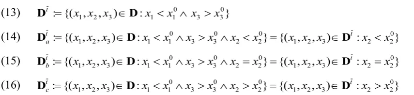
Now, we study the following (calculus-of-variations) problem. Assume that Assumptions 1-3
are satisfied (and, thus, 0
) 0
( X
X is given) and that the path-destination (at time t ) is
determined, i.e. X(t) Xt is given. There exist different paths that connect X0 and Xt in
Euclidean space (cf. Figure 1). A path is “admissible” if it is continuous (cf. Assumption 2b)
and if it connects X0 and Xt. The functional (3) associates each of these admissible paths
with a certain magnitude of structural change costs c0t . We search for an answer to the
following question: ‘Which of the admissible paths is associated with minimal structural
change costs (c0t)?’ That is, we want to find the (admissible) path that minimizes the structural
change costs c0t. Lemma 1 provides the solution of this problem.
Figure 1. The calculus-of-variations problem solved by Lemma 1.
- insert Figure 1 here -
Lemma 1. Assume that Assumptions 1 to 3 are satisfied and that the path-destination at time
t > 0 is given, i.e. X(t) Xt (x1t,x2t,...xnt)Rn. Under these conditions, any monotonous
(and continuous) development path (cf. Definition 2) that connects X and 0 X (in Euclidean t
space) is associated with minimal structural change costs c0t (cf. Definition 3).
For a proof of Lemma 1 you could apply the theorems of the calculus of variations (see, e.g.,
Gelfand and Fomin (1963), Chapter 15). In the APPENDIX, we provide a more detailed
(geometrical) proof, which uses the techniques familiar to calculus of variations. This detailed
proof provides us with lemmas and interpretations that are helpful for proving and
understanding the properties of the minimal-costs paths that will be discussed later.
Simply speaking, Lemma 1 states that if we want minimal structural change costs, it does not
matter which path we take from X0 to t
X as long as it is monotonous (and per assumption
12
Note that since Lemma 1 is valid for any Xt n R
, we could formulate it more generally, i.e.
we can omit the reference to X0 and Xt, as follows: any monotonous path (in Euclidean
space) is associated with minimal structural change costs.
Note that we assume throughout the paper that X(t) is C1 (see, e.g., Definition 3 and Assumption 3), i.e. the development path has a certain degree of smoothness. This argument is
valid, since we study here only long-run trend paths, i.e. the smoothness of X(t) is per
definition (of the term ‘long run trend’.
Obviously, if Xt X0, the structural change costs-minimizing strategy (for ‘moving’ from
0
X to t)
X is: stay in X0 for all t[0,t], i.e. no structural change at all! Such a ‘path’ is per
Definition 3 monotonous.
5. Monotonous Paths in the Three-Sector Framework when the Path-Destination is
Determined by Meta-Theorems 1 and 2
In this section, we prove the following lemma. As we will see later, this lemma and Lemma 1
imply jointly the existence of a structural change costs-minimizing path given Meta-theorems
1 and 2.
Assumption Set 1. We consider the three-sector economy (n = 3) over the period [0,), where
t = 0 denotes the present. Assume that the initial structure of the economy (at t = 0) is given by
the vector
(4) ( , ,. 30) 0
2 0 1 0
x x x
X R3.
Let t denote a future time point, i.e.
(5) t(0,)
and X denote the structure of the economy at t , where t
(6) Xt (x1t,x2t,x3t) 3
R
Let Meta-theorems 1 and 2 be valid, i.e. assume that
(7) x1t x10 x3t x30
Moreover, let the vectors X and 0 X satisfy the following conditions t
13
Lemma 2. a) Let the Assumption Set 1 be valid. Then, there exists a path
)) ( ), ( ), ( ( )
( 1* *2 3*
* t x t x t x t
X , t[0,t], that has the following characteristics
(I) t[0,t]i{1,2,3} 0 xi*(t)1 ( ) ( ) *3( ) 1
* 2 *
1 t x t x t x
(II) t[0,t] *( )
t
X is continuous in t
(III) t[0,t] X*(t) is monotonous in t
(IV) X*(0) X0
(V) t
X t X*( )
(VI) t'(0,t):t[0,t') x*2(t)x20
b) Let the Assumption Set 1 be valid. Then, for some XtR3 (satisfying (8)) there does not
exist a path X*(t)(x1*(t),x2*(t),x3*(t)), t[0,t], satisfying the conditions (I), (II), (III), (IV),
(V) and (VI’), where
(VI’) t'(0,t):t[0,t') dx2*(t)/dt0.
c) Let the Assumption Set 1 be valid. Then, for some Xt R3 (satisfying (8)) there does not
exist a path X*(t)(x1*(t),x2*(t),x3*(t)), t[0,t], satisfying the conditions (I), (II), (III), (IV),
(V) and (VI’’), where
(VI’) ' (0, ): [0, ') *( )/ 0
2
t t t t dx t dt .
We choose here a rather ‘informal’ way of proving Lemma 2 allowing us to discuss the aspects
being proven and derive some corollaries that will be of interest in Section 6. The proof is
structured as follows: first, we show that the path characterized by Lemma 2 is located in a
subset (D) of a plane in R3 and that the path-destination (which is determined by Meta-theorems 1 and 2) is located in a subset (Dt) of D; then, we partition the subset Dt and show that (a) a
path characterized by (VI) can be constructed to any location in any partition while satisfying
requirements (I)-(V) and (b) a path characterized by (VI’) or (VI’’) cannot lead to some of the
partitions if (I)-(V) are satisfied.
We start the proof by defining the path P* as follows: (9) P*:{X*(t)R3:t[0,t]}
Lemma 2 states that P* satisfies the condition (I) among others. Condition (I) states that the path P* is located in the set
(10) D:={( , , ) 3: 3
2
1 x x R
14
In other words,
(11) P* D
Thus, when searching for P* satisfying the characteristics (I)-(VI), we do not need to analyze
the whole R3, but can restrict our attention to D.
As discussed by Stijepic (2015), (10) states that D is a standard 2-simplex, which is a subset of
a plane in R3; in particular, D is a triangle with the vertices V1:=(1,0,0), V2:=(0,1,0) and V3:=(0,0,1) in the Cartesian coordinate system (see Figure 2).
Figure 2. The standard 2-simplex (D) in the Cartesian coordinate system.
- insert Figure 2 here -
Henceforth, we depict D without the coordinate system, as depicted in Figure 3.
Figure 3. The standard 2-simplex (D) depicted without the coordinate system.
- insert Figure 3 here -
(4), (6), (8) and (10) imply
(12) X0D Xt D
(11), (12), (IV) and (V) imply that the path P* connects 0
[image:15.595.71.499.598.696.2]X and Xt on D (cf. Figure 4).
Figure 4. An example of the path P*.
- insert Figure 4 here -
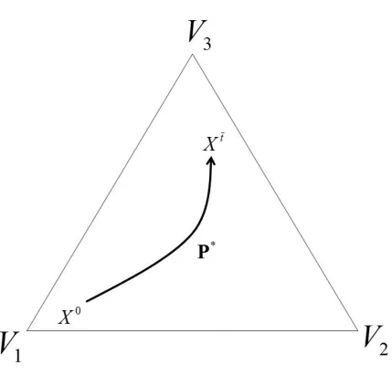
Given an initial state X0D, we define the set Dt and its partitioning ( t a
D , t
b
D , t
c
D ) as
follows :
(13) : {( , , ) : 3 30}
0 1 1 3
2
1 x x x x x x
x
t
D D
(14) : {( , , ) : } {( 1, 2, 3) : 2 20}
0 2 2 0 3 3 0 1 1 3 2
1 x x x x x x x x x x x x x
x t
t
a D D
D
(15) Dbt :{(x1,x2,x3)D:x1x10x3 x30x2x20}{(x1,x2,x3)Dt :x2 x20}
(16) : {( , , ) : } {( 1, 2, 3) : 2 02}
0 2 2 0 3 3 0 1 1 3 2
1 x x x x x x x x x x x x x
x t
t
c D D
D
As we can see, Dt is the set of all points (on D) satisfying Meta-theorems 1 and 2 (cf. (7) and
(13)). Dtand its partitioning ( t a
D , t
b
D , t
c
15 Figure 5. The set Dt and its partitioning.
- insert Figure 5 here -
Note.A and C are open sets. The sets associated with segments do not contain the end-points of the
line-segments, e.g. the set 𝑋𝑌̅̅̅̅ associated with the line-segment connecting the points X and Y does not contain the
points X and Y.
Note that (10) and (14)-(16) imply that t a
D , t
b
D and t c
D are pairwise disjoint and their union
is equal to Dt. Thus, ( t a
D , t
b
D , t
c
D ) is a partitioning of Dt, i.e.
(17) t
a
D Dtb Dtc=Dt
(18) i{a,b,c}j{a,b,c}\i Dti Dtj ∅
(6), (7), (12) and (13) imply that Xt is located in Dt, i.e.
(19) Xt Dt
Overall, (17)-(19) imply that Xt is located in one and only one of the sets t a
D , t
b
D and t c
D .
Thus, we can distinguish between three cases: (1.) Xt t a
D , (2.) Xt t b
D , and (3.) Xt
.
t c
D
Before analyzing these cases, we introduce the following vector angle definition, which allows
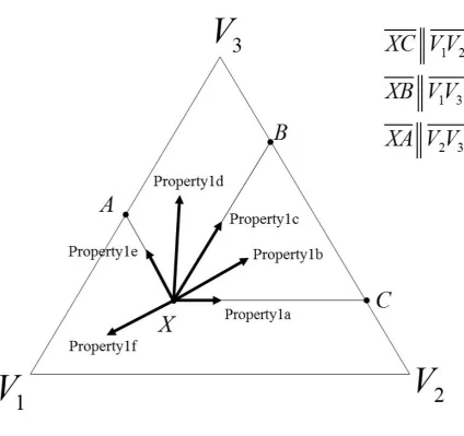
us to analyze the dynamics on D by referring to vector angles.
Definition 4. Let X be a point on D and D(X) be a vector indicating the direction of movement
associated with point X. (For example, X may be a point on a curve/trajectory on D and D(X)
a tangential/directional vector associated with point X.) The vector angle δ(D(X)) is the angle
between D(X) and the simplex-edge V1V2, i.e. δ(D(X))∶= ∠(D(X),V̅̅̅̅̅̅1V2).
This definition and the definition of D imply the following properties of a directional vector D
on the simplex D.
Property 1.a) If δ(D(X)) = 0°, the movement indicated by vector D(X) is characterized by a
decrease in x1, an increase in x2 and a constant x3.
b) If 0 < δ(D(X)) < 60°, the movement indicated by vector D(X) is characterized by a decrease
in x1, an increase in x2 and an increase in x3.
c) If δ(D(X)) = 60°, the movement indicated by vector D(X) is characterized by a decrease in
16
d) If 60° < δ(D(X)) < 120°, the movement indicated by vector D(X) is characterized by a
decrease in x1, a decrease in x2 and an increase in x3.
e) If δ(D(X)) = 120°, the movement indicated by vector D(X) is characterized by a constant x1,
a decrease in x2 and an increase in x3.
f) If δ(D(X)) > 120°, the movement indicated by vector D(X) is characterized by an increase in
x1 or a decrease in x3.
Figure 6 illustrates Property 1.
Figure 6. Examples of vectors characterized by Property 1.
- insert Figure 6 here -
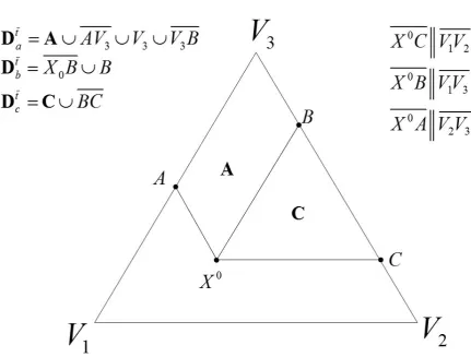
Henceforth, we use Definition 4 and Property 1 to characterize the path P* as follows. The path
P* assigns to each t[0,t] an X*(t) (cf. (9)). We can assign to each X*(t) a directional vector D(X*(t)) indicating the direction of movement along the path P* at the point X*(t)
(cf. Definition 4). (In case of differentiable functions, i.e. if *( )
t
X is differentiable with respect
to t, D(X*(t)) can be interpreted as the tangential (or directional) vector at point X*(t) of the
curve X*(t), t[0,t], associated with the path P*.) Moreover, via Definition 4, we can measure the vector angle ( ( *( )))
t X D
and identify the changes in (x1,x2,x3) at the point
), (
* t
X i.e. we can identify the signs of *( )/ ,
1 t dt
dx dx*(t)/dt
2 and dx (t)/dt *
3 at each point of
P*.
Now, we return to the three cases. First, we analyze case 1, i.e.
(20) t
X t
a
D
(6), (14) and (20) imply
(21) 0
1
1 x
xt 0
2
2 x
xt 0
3
3 x
xt
(21) states that at the destination Xt of the path P*, x3 (x1 and x2) is (are) greater (smaller) than in the initial state X0. (III) and Definition 3 imply that, thus, x3 (x1 and x2) must grow (decrease) monotonously along the path P* (cf. Remark 1), i.e.
(22) t[0,t) dx1*(t)/dt0dx2*(t)/dt0dx*3(t)/dt0
17
where (23) states that x1, x2 and x3 must change over time (according to (21)), since otherwise (21) cannot be satisfied.
By using Property 1, we can translate (22) and (23) as follows:
(24) t[0,t) 60(D(X*(t)))120
(25) t[0,t)60(D((X*(t)))120
By now, we have shown that if (20) is true, P* must satisfy (24) and (25) due to the monotonicity requirement (III) among others. Moreover, (25) does not prohibit (D((X*(0)))
= 60° or for some t, (D((X(t)))120. That is, we can construct a path P**:{X**(t)D:
]} , 0 [ t
t that can be partitioned into two linear segments
(26) PI**:{X**(t)P**:t[0,t')}
(27) PF**:{X**(t)P**:t[t',t]}
where the initial path-segment (PI**) is characterized by a tangential vector angle of 60°, i.e.
) ' , 0 [ t t
( (( **( )))60
t X D
, and the final path-segment ( **
F
P ) is characterized by a
tangential vector angle of 120°, i.e. t[t',t) (D(X**(t)))120, while being consistent with (24) and (25) and all the other requirements (e.g. (IV) and (V)) listed in Lemma 2. That is:
(28) P**:{X**(t)D:t[0,t]}X**(0)X0DX**(t)Xt Dat (t[0,t')
))) ( ( (D X** t
60)(t[t',t)(D(X**(t)))120)
An example of the path P** is depicted in Figure 7.
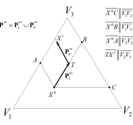
Figure 7. An example of P**.
- insert Figure 7 here -
This discussion states that it is possible to construct a path P** that has (a) the characteristics (I)-(VI) and (b) an initial segment ( PI** ) that is characterized by a vector angle
60 ))) ( ( (D X** t
(over the initial phase [0,t')). However, this discussion does not tell us
how long the initial segment PI** is (given a X0 and a Xt ); in other words, we have not
determined t’ in (26)-(28). The magnitude of t’ will be later of importance (when determining
the length of the optimal policy).
We use Figure 7 to illustrate the geometrical derivation of the length of PI** for any X0
D
and any Xt t a
18
parallel to the simplex-edge V1V3. Moreover, given a Xt Dta, we construct a line-segment
going through t
X and being parallel to the simplex-edge V2V3. Let T be the point of intersection between the two line-segments. PI** is the linear path from
0
X to T; PF** is the
linear path from T to Xt; P** is the union of PI** and PF**. The length of PI** is equal to the distance between X0 and T. As we can see in Figure 7, the length of PI** is equal to the distance
between Xt and X0A and is non-trivial except in the limiting case of Xt X0A. (As
implied by Figure 2, the distance between Xt and X0A depends on the difference x1 x10,
t
where Xt X0A for x1t x10 .) The limiting case x1t x10 is not of interest (cf.
Meta-theorem 1). If the length of PI** is non-trivial and if the velocity of structural change (i.e. the
velocity of movement along PI**) is not infinitely large, the fact that the length of
* *
I
P is
non-trivial implies that t’ is non-trivial, i.e. the duration of movement along PI** is non-trivial.
Finally, note that (24) states that t[0,t), P* must not be characterized by (D(X*(t)))
60 or (D(X*(t)))120 (in case 1, i.e. if Xt t a
D ). Moreover, the movement along
path-segment PF** is characterized by a decreasing manufacturing share x2 and a growing services share x3 (cf. (28), Figures 2 and 7 and Property 1e).
Overall, by now, we have considered case 1, i.e. we assumed that Xt t a
D . We have shown
that in this case:
(A) a monotonous and continuous path (X**(t),t[0,t]) can be constructed that
(i) connects X0D and t a t
X D and
(ii) is characterized by (D(X**(t)))60 over some initial period [0,t') of
non-trivial length;
(B) there does not exist a continuous and monotonous path (X**(t),t[0,t]) that
(i) connects X0D and XtDta and
(ii) is characterized by (D(X**(t)))60 or (D(X**(t)))120 over some
initial period [0,t') of non-trivial length.
19
(C) in case 2, i.e. if Xt t b
D , a continuous and monotonous path (X**(t),t[0,t])
that connects X0D and Xt t b
D must be characterized by (D(X**(t)))60
) , 0 [ t t ;
(D) in case 3, i.e. if Xt t c
D :
(a) a monotonous and continuous path (X**(t),t[0,t]) can be constructed that
(i) connects X0D and Xt t c
D and
(ii) is characterized by (D(X**(t)))60 over some initial period
) ' , 0
[ t of non-trivial length;
(b) there does not exist a continuous and monotonous path (X**(t),t[0,t])
that
(i) connects X0D and Xt t c
D and
(ii) is characterized by (D(X**(t)))60 over some initial period
) ' , 0
[ t of non-trivial length.
These facts (i.e. points (A)-(D)) imply that in all three cases, only an initial angle of 60°, i.e.
60 ))) 0 ( ( (D X**
, ensures that we can reach our destination along a monotonous (and
continuous) path. (Moreover, the vector angle (D(X**(t)))60 can be sustained over some
initial period [0,t') of non-trivial length while ensuring that the path is monotonous and
continuous and the destination is reached.) Any other initial vector angle cannot ensure in all
cases that we can reach the destination along a monotonous and continuous path. For example,
if the initial vector angle is equal to 80°, i.e. (D(X**(0)))80, a monotonous and continuous
path can be constructed to a destination in t a
D but not to a destination in t c
D . Finally, note that
Property 1 states that (D(X**(t)))60 for [0,t') means that the employment share of
manufacturing is constant over the period [0,t'). Moreover, ( ( **( )))
t X D
60 for [0,t')
means that the employment share of manufacturing is not constant over the period [0,t'). These
facts prove Lemma 2.
Note that the proofs of the following facts are analogous to the corresponding proofs discussed
in this section: (a) the length of PI** and, thus, the magnitude of t’ depends on the difference
0 3
3 x
xt if Xt t c
D ; (b) t’ = t if Xt t b
D ; (c) if Xt t c
D , the path-segment **
F P is
20
We provide now an interpretation of Lemma 2.
6. Discussion
6.1. Implications of Lemmas 1 and 2: Cost-Minimizing Development Strategy
We can use Lemmas 1 and 2 to derive the optimal structural change policy as follows. Lemma
1 states that monotonous development paths minimize the structural change costs. Lemma 2a
states that for any path destination Xt (cf. (V)) satisfying Meta-theorems 1 and 2 (cf. (7)),
there exists a monotonous path (cf. (III)) that is characterized by a constant manufacturing
employment share over some initial phase [0,t’) (cf. (VI)); moreover, Lemma 2a implies that
this path is characterized by a monotonously growing (decreasing) services (agricultural) share
(cf. (7), (III) and Definition 3). Lemmas 2b and 2c state that if the social planer does not choose
a policy that ensures a constant manufacturing share over the initial development phase (cf.
(VI’)and (VI’’)), then the economy may not be able to reach its destination along a monotonous path (cf. (III)).
Jointly, Lemmas 1 and 2 imply that an underdeveloped country not knowing the exact
destination of its structural change path should choose the following policy:
(a) decreasing agricultural share,
(b) constant manufacturing share and
(c) increasing services share.
This policy is consistent with the theoretical and empirical literature consensus on the
path-destination of a developing economy (cf. Meta-theorems 1 and 2) and minimizes the country’s
future structural change costs.
6.2 On the Optimal Duration of Policy (a)-(c)
Lemma 2 states that the structural policy (a)-(c) is only optimal over the initial phase of
development, which is in our model denoted by the time-interval [0,t’). As implied by the
discussion (cf. Section 5), the length of this phase (which can be derived from the length of the
initial path-segment PI**) depends on the differences between the initial and the destined
agricultural and services employment shares (x1t x10 and x3 x30
t
). Since, in general, these
differences are relatively large in an underdeveloped yet developing country, it seems that
policy (a)-(c) is optimal over a relatively long phase, as demonstrated by the following example
21
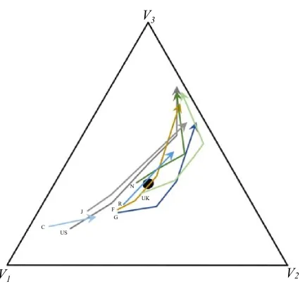
The USA accomplished their structural transformation from an agricultural to a services
economy over a period of ca. 170 years, as illustrated by Figure 8, which depicts among others
the US structural change over the period 1820-1992. Figure 8 implies that it is possible to
construct a linear line-segment that (a) is approximately parallel to the V1V3 edge of the simplex and (b) connects the initial point (representing 1820) and the last point (representing
1992) of the US trajectory.3 In our modeling framework, this line-segment is denoted by **
I P
(cf. Figure 7) and represents policy (a)-(c), i.e. a structural change path that is characterized by
a constant manufacturing share (over the period 1820-1992). Thus, our results imply that in the
case of the USA, policy (a)-(c) would have been optimal over a period of ca. 170 years and
would have avoided the costs of industrialization (e.g. the declining health of the population
and the problems with urbanization) and the costs of de-industrialization (e.g. urban decline
and unemployment). Of course, these arguments only refer to the structural change
cost-minimization problem and neglect other aspects of optimal structural policy discussed in
Section 2.
Figure 8. Labor allocation trajectories for the USA, France, Germany, Netherlands, UK,
Japan, China, and Russia.
- insert Figure 8 here -
Notes. Data source: Maddison (1995). The black dot represents the barycenter of the simplex. Abbreviations: C
– China, F – France, G – Germany, J – Japan, N – Netherlands, R – Russia, US – United States, UK – United Kingdom. Data points (years in parentheses): USA (1820, 1870, 1913, 1950, 1992), France (1870, 1913, 1950,
1992), Germany (1870, 1913, 1950, 1992), Netherlands (1870, 1913, 1950, 1992), UK (1820, 1870, 1913, 1950,
1992), Japan (1913, 1950, 1992), China (1950, 1992), Russia (1950, 1992).
6.3 Optimal Policies Following Policy (a)-(c)
As discussed in Sections 5 and 6.2 (in the case of the USA), policy (a)-(c), which is represented
by path-segment PI**, may be optimal over a relatively long period. However, the discussion
in Section 5 has shown that this is a special case and in general, policy (a)-(c) must be followed
by a de-industrialization accompanied by a tertiarization or an industrialization accompanied
by an agricultural decline (cf. the discussion of path-segment PF**) if we seek to minimize the
3 Note that Figure 8 depicts the development of the USA until 1992. Since 1992, the USA have come even closer
to the simplex-edge V1V3 such that the line-segment connecting their present-day’s location and their initial (i.e.
22
structural change costs. Thus, policy (a)-(c) does not only minimize the structural change costs
but also allows for a postponing of the industrialization/de-industrialization decision to a later
phase of development, where additional information on the global environment may be
available.
6.4 Comparison of Policy (a)-(c) to the Standard Structural Policies
As discussed in Section 2, the previous literature implies different structural change strategies.
We compare now these strategies with policy (a)-(c).
Our results imply that the ‘Washington Consensus strategy’ (in particular, trade liberalization)
emphasizing the agricultural sector in the early stages of development is associated with high
structural change costs. It contradicts the policy aspect (a) (‘decreasingagricultural share’). In
general, nearly all highly developed countries are characterized by relatively low agricultural
shares (cf. Figure 8). Thus, the increases in the agricultural share (induced by the Washington
Consensus strategy) must be reversed at some later stages of development, which causes
unnecessary structural change costs.
Moreover, the Kaldorian strategy of emphasizing the manufacturing sector, which has been
pursued by many socialist countries (e.g. China) contradicts the policy aspect (b) (‘constant
manufacturing share’). Examples of the negative effects of a manufacturing sector emphasis are well known from the history (e.g. the food shortages in USSR and China) and the present
experiences (e.g. the environmental pollution in China) of socialist countries. Many
highly-developed countries (e.g. UK) went through severe phases of de-industrialization, which were
characterized by unemployment, urban decline and political/social instabilities. These crises
can be avoided if an overshooting of the manufacturing sector is avoided and, in particular, the
manufacturing share (in GDP or employment) is kept approximately constant as suggested by
policy (a)-(c). However, our results do not prohibit a restructuring of the manufacturing sector
towards more modern products and technologies, while keeping the employment share of the
manufacturing sector constant. Thus, policy (a)-(c) is rather a policy of restructuring the
manufacturing sector than a policy of increasing its share/size disproportionately.
Finally, it seems that the ‘recent Indish’ strategy, which refers to a transformation from an
agricultural to a services economy, is consistent with policy (a)-(c).
6.5 A Comparison of Empirically Observed Structural Change Paths and Policy (a)-(c)
Discussing and comparing the structural change paths and their costs across countries is a
23
and simple applicability of the concepts developed in our paper, we briefly discuss here the
long-run data on structural changes in present-day’s most developed and emerging countries.
By using Property 1, we can analyze the monotonicity features of this long run data. This
property and Figure 8 imply that the countries’ agricultural (services) shares decreased
(increased) in the long run, thus being consistent with the aspects (a) and (c) of the policy
derived in our paper. Moreover, Figure 8 shows that Germany and UK had developed the
highest manufacturing shares over time (as implied by Property 1).4 UK has reduced the employment share again, resulting in a very curved5 structural change path. This contradicts policy (a)-(c), and our measure c0t implies that the structural change costs associated with this
path are relatively high. Whether Germany will face high overall structural change costs
depends on its future development (i.e. the future degree of de-industrialization). Moreover,
Figure 8 reveals that China has developed against policy (a)-(c) by pursuing a strong
industrialization program.
7. Concluding Remarks
The growth and development process is characterized by massive structural change, which
generates high costs for the society and the economy ranging from pollution to unemployment.
In this paper, we have derived the properties of the development path that minimizes the
structural change costs in the three-sector framework depending on the destination of the path,
where we assumed that the structural change costs increase with the strength of structural
change. Moreover, we have discussed the structural change theories and the empirical evidence
and derived the literature consensus/prediction regarding the destination of the structural
change path of a today’s underdeveloped economy. The consensus statements are crude and
qualitative such that the set (D𝑡̅) of potential destinations implied by the consensus is relatively great. For this reason, among others, we had to apply qualitative/geometrical modeling
techniques for deriving the structural change costs-minimizing policy in a today’s
underdeveloped country when assuming that the country’s destination is located in the set D𝑡̅. We have shown that the cost-minimizing policy is characterized by a decreasing agricultural
employment share, a constant manufacturing employment share and a growing services
4 The magnitude of the manufacturing employment share in Figure 8 is indicated by the closeness to vertex V
2
(see also Stijepic (2015)). As we can see, the trajectories of Germany and UK come very close to vertex V2.
5 In particular, the fact that the path is curved with respect to the V
1V3-edge of the simplex is relevant. It implies
that the manufacturing share increased strongly (as the economy moved away from the V1V3-edge) and, then,
24
employment share. Finally, we applied this theoretical result for evaluating (a) the standard
development strategies and (b) some historically observed structural change paths in developed
economies regarding the structural change costs they generate (cf. Section 6). As we have
shown, our results imply among others that the standard development strategies generate
relatively high structural change costs and that, e.g., UK, Germany and China have chosen
structural change paths that are (potentially) associated with high structural change costs.
While these applications are only brief demonstrations of the applicability of our results, future
research could focus on more elaborate (empirical) studies of these aspects. For example,
countries could be grouped into groups with relatively high and relatively low structural change
costs and the properties of these groups (e.g. prevalence of crises, political regime, etc.) could
be analyzed. Moreover, the importance of the structural change costs in relation to the other
effects of structural policies discussed in Section 2 for welfare and growth could be estimated.
References
Baumol, W.J., 1967. Macroeconomics of unbalanced growth: the anatomy of urban crisis.
American Economic Review 57(3), 415–426.
Baumol, W.J., Batey-Blackman S.A., Wolf E.N., 1985. Unbalanced growth revisited:
asymptotic stagnancy and new evidence. American Economic Review 57(3), 415–426.
Demirgüç-Kunt, A., Levine, R. (Eds.), 2004. Financial structure and economic growth: a
cross-country comparison of banks, markets, and development. MIT Press.
Foellmi, R., Zweimüller, J., 2008. Structural change, Engel’s consumption cycles and Kaldor’s facts of economic growth. Journal of Monetary Economics 55(7), 1317–1328.
Gelfand, I.M., Fomin, S.V., 1963. Calculus of variations. Dover Books on Mathematics.
Greenwald, B., Stiglitz, J.E., 2006. Helping infant economies grow: foundations of trade
policies for developing countries. American Economic Review 96(2), 141–146.
Hadass, Y.S., Williamson, J.G., 2003. Terms‐of‐trade shocks and economic performance,
1870–1940: Prebisch and Singer revisited. Economic Development and Cultural Change 51(3),
629–656.
Harrison, A., Rodríguez-Clare, A., 2010. Trade, foreign investment, and industrial policy for
developing countries. In: D. Rodrik and M. Rosenzweig (Eds.), "Handbook of Development
Economics", Edition 1, Volume 5, Number 6, Elsevier.
Herrendorf, B., Rogerson, R., Valentinyi, Á., 2014. Growth and structural transformation.
In: Aghion P. and S.N. Durlauf (Eds.), “Handbook of Economic Growth”, Volume 2B, Elsevier
25
Kongsamut, P., Rebelo, S., Xie, D., 2001. Beyond balanced growth. Review of Economic
Studies 68(4), 869–882.
Krüger, J.J., 2008. Productivity and structural change: a review of the literature. Journal of
Economic Surveys 22(2), 330–363.
Maddison, A., 1995. Monitoring the world economy 1820–1992. OECD Development Centre.
Moro, A., 2012. The structural transformation between manufacturing and services and the
decline in the US GDP volatility. Review of Economic Dynamics 15(3), 402–415.
Ngai, R.L., Pissarides, C.A., 2007. Structural change in a multisector model of growth.
American Economic Review 97(1), 429–443.
Robinson, J.A., 2009. Industrial policy and development: a political economy perspective.
Working paper prepared for the 2009 World Bank ABCDE conference in Seoul June 22-24.
Rodrik, D., 2006. Goodbye Washington consensus, hello Washington confusion? A review of
the World Bank's economic growth in the 1990s: learning from a decade of reform. Journal of
Economic Literature 44(4), 973–987.
Rodrik, D., Rosenzweig, M. (Eds.), 2010. Handbook of Development Economics. Elsevier.
Schettkat, R., Yocarini, L., 2006. The shift to services employment: a review of the literature.
Structural Change and Economic Dynamics 17(2), 127–147.
Silva, E.G., Teixeira, A.A.C., 2008. Surveying structural change: seminal contributions and a
bibliometric account. Structural Change and Economic Dynamics 19(4), 273–300.
Stiglitz, J.E., Lin, J.Y., Monga, C., 2013. The rejuvenation of industrial policy. Policy
research working paper No. WP6628.
Stijepic, D., 2011. Structural change and economic growth: analysis within the partially
balanced growth-framework. Südwestdeutscher Verlag für Hochschulschriften, Saarbrücken.
An older version is available online: http://deposit.fernuni-hagen.de/2763/.
Stijepic, D., 2015. A geometrical approach to structural change modelling. Structural Change
and Economic Dynamics 33, 71–85.
Stijepic, D., 2016a. A topological approach to structural change analysis and an application to
long-run labor allocation dynamics. Munich Personal RePEc Archive working paper No.
74568.
Stijepic, D., 2016b. Positivistic models of long-run labor allocation dynamics. Munich
Personal RePEc Archive working paper No. 75050.
Uy, T., Yi, K.-M., Zhang, J., 2013. Structural change in an open economy. Journal of