Extra Nodes Added on the Solid/Liquid Interface to Solve the Mass
Transfer Problem in a Directional Solidification Process
Yau-Chia Liu and Long-Sun Chao
Department of Engineering Science, National Cheng Kung University, No.1, Ta-Hsueh Road, Tainan 701, Taiwan, R.O.China
In a directional solidification process, since the liquid solubility is higher than the solid one, the surplus solute will be released from the solid/liquid interface into the liquid, which is the main source of increasing the liquid solute. The release of solute at the moving interface is like that of latent heat. Except the growth rate, the release of extra solute also depends on the liquid concentration at the interface, which is not fixed. Consequently, the numerical treatment of the solute release is not so easy as that of the latent-heat one. If the effect of solute release is not handled appropriately, the concentration solutions will diverge very easily. In this paper, extra nodes added on the solid/liquid interface in a fixed grid system are proposed to solve the mass transfer problem in the directional solidification process. A one-dimensional problem is firstly used to test the proposed method. The computing results are compared with those of other fixed grid methods and the analytical solutions from the literature. Finally, the feasibility of the proposed method is further testified by applying it to solve the concentration field of the crystal growth of GaAs in a Bridgman furnace. [doi:10.2320/matertrans.MB200711]
(Received March 1, 2007; Accepted June 1, 2007; Published July 19, 2007)
Keywords: mass transfer, directional solidification, fixed grid system, extra node and crystal growth
1. Introduction
In the recent years, semiconductor is generally applied in integrated circuits or microelectronic parts. Therefore, it is very important to make semiconductor materials with high purity, high homogeneity and good crystal quality are in highly demands. Homogeneity is one of the key factors that can affect the quality of single crystal materials. Good homogeneity represents the well-mixed degree of dopant distribution. However, the temperature field, velocity field, and the profile of solid/liquid interface mainly affect the dopant concentration distribution as the crystal grows. Consequently, how to effectively control the heat and mass transfers and the shape of solid/liquid interface in the crystal growth system is the key point to control the crystal quality. For solving the crystal growth problem, if flow field is known, it seems that the concentration field can be solved numerically without too much difficulty by putting the velocity distribution into the concentration equation. How-ever, it is really not so simple to solve the concentration field of dopant in the melt during the crystal growth of a semiconductor material. In the crystal growth, because the liquid solubility of dopant is higher than the solid one, the surplus solute will be released from the solid/liquid interface into the liquid, which is the main source of increasing the liquid solute. The release of solute at the moving interface is like that of latent heat. The release of latent heat per unit volume depends on the growth rate and the latent heat and the latter one is a fixed value. However, except the growth rate, the release of extra solute is also related to the liquid concentration at the interface, which is not a fixed one. Consequently, the numerical treatment of the solute release is not so easy as that of the latent-heat one. If the effect of the solute release is not handled appropriately, the concentration solutions will diverge very easily.
To solve the temperature field in a solidification process, the numerical methods can be generally divided into two kinds: the fixed domain method1–4,26)and the front tracking
method.5–9) The fixed domain method treats the liquid and solid phases as a computing domain. The temperature fields of both phases are solved together. The latent heat is put into the specific heat or heat source term or the enthalpy is used instead of the temperature in the numerical calculation. In the front tracking method, the temperature distributions of solid and liquid phases are solved separately and they are linked by the Stefan condition and the solidification temperature at the solid/liquid interface. At every time step, the location of the interface needs to be traced out. Originally, the grid system for this method is not fixed and needs to be changed every time step for the new interfacial location, which makes the numerical computation complicated. Recently, the method is applied to the fixed grid system. In a fixed grid system, the main disadvantage in the use of the front tracking method is that it is difficult to precisely track the interface. Laboniaet al.5)delivered a scheme to solve this problem. They used an explicit interface-tracking scheme that involves the straight-line reconstruction and advection of the interface on a fixed grid. Furthermore, Li et al.6) utilized a cubic-spline recon-struction for determining the marker points and improved the marker points at the boundary. The results for solidification front locations and temperature are as well as those using an adaptive grid generation scheme.7)
In solving the concentration field in a solidification process as mentioned above, it is not so simple as in the heat transfer analysis since the variable of interfacial concentration is involved in the calculation of the solute release. Voller et al.10)treated the solute release at the interface as a source term in the concentration equation, in which an extrapolation procedure was used to calculate the interface concentration. A fixed grid single domain approach was utilized to obtain the concentration solutions, which are averaged over the computational cells. With the similar method, Timchenkoet al.11)extrapolated the interface concentration exponentially, according to the one-dimensional steady solution. Lan et al.12)proposed a finite volume (FV)/ Newton’s method for the calculation of solute transfer in directional solidification. Special Issue on Solidification Science and Processing for Advanced Materials
Due to the unknown and irregular growth interface, the rz coordinates are transformed into the general curvilinear ones. Compared to those of the Galerkin finite element method (FEM),13,14)the results showed the global conservation could be preserved in FVE and the FEM cannot satisfy the global conservation very well in coarse meshes. Stelianet al.15,16)
used the free-surface enhancements introduced by the FIDAP package to modeling the solute transport at the solid/liquid interface and the computed results are in good agreement with those from the experimental analysis.17)
The key problem of handling the solute release at the solid/liquid interface is how to obtain the interface concen-tration. Generally, this can be solved by two basic methods, one is the front tracking method and the other is the extrapolation scheme. The former one is more accurate and complicated numerically than the latter one. Though the extrapolation method is easier, it would lead to the inaccurate or even the diverging solution if the method is not handled appropriately. For the directional solidification problem, an intermediate method between these two schemes is proposed in this work to solve the solute release problem at the interface, in which extra nodes are added at the interface to obtain the interface concentrations without changing the original fixed grid system. This method is similar to those front tracking methods used in a fixed grid for solving the temperature field in a solidification process. The interface temperature is the melting temperature, which is known. However, the interface concentration is unknown and plays an important role in the calculation of solute release. To test the proposed method, a one-dimensional problem is firstly used. The computing results are compared with those of other fixed grid methods and the exact solutions from the literature. Finally, the feasibility of the method is further testified by using a crystal growth problem.
2. Problem Description
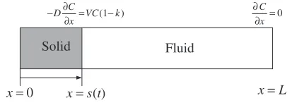
The considered physical model is a directional growth along the x-axis in a limited length, as shown in Fig. 1. In the figure, L is the total length of the physical model, V is the growth rate of solid/liquid interface andsðtÞis the position of solid/liquid interface. C and D are the liquid concentration and diffusivity, respectively.
To simplify the problem, the following assumptions are made firstly for building the mathematical model, in which the liquid concentration field can be solved solely:
1. The solute diffusion in solid is ignored.
2. The growth rate of solid/liquid interface, V, is constant. From the physical model and the assumptions stated above, the governing equation and the initial and boundary conditions can be given as follows.
(1) Governing equation
@C
@t ¼D
@2C
@x2 ð1Þ
(2) Initial condition
Cðx;t¼0Þ ¼C0 ð2Þ
whereC0 is the initial concentration.
(3) Boundary condition
x¼sðtÞ ¼Vt; D@C
@x ¼VCð1kÞ ð3Þ x¼L; @C
@x ¼0 ð4Þ
wherekis the equilibrium distribution coefficient.
3. Numerical Method
In the paper, the numerical method is the finite difference method. In the formulation of the difference equation, the centered difference is utilized for the space derivative and the backward difference is for the time derivative. In solving the solute redistribution, extra nodes are added at the solid/liquid interface and their difference formulations can help to obtain the interface concentrations, from which the solute release can be estimated accurately. For those nodes not involved in the phase change, the finite-difference formulation of the governing equation can be written as
Cniþ1Cni
t ¼D
Cinþþ112Cinþ1þCniþ11
x2 ð5Þ
where the superscript n is the index of time and the subscript i is the index of space grid.
In Fig. 2, the solid/liquid interface is located between node i and i-1 att¼tnþ1. A node, node int, representing the
interface is added and the difference formulations for node int and node i need to be re-derived. The shadow areas shown in Fig. 2(a) and 2(b) are the control volumes of these two nodes. In the control volume of node int, xint is the distance between node i and int andxint=2is the width of the control volume. For the control volume, the solute balance can be written as
@C
@t
nþ1
int
Axint
2 ¼ ðJ1þJ2ÞA ð6Þ where A is the area of cross section.J1 andJ2 are the solute
fluxes entering from the left and the right sides of the control volume and can be expressed as
J1¼VCintnþ1ð1kÞ ð7Þ
J2¼D
Cniþ1Cintnþ1
xint
ð8Þ
For the control volume of node i (Fig. 2(b)), the solute balance can be written as
@C
@t
nþ1
i
Axþxint
2 ¼ ðJ3þJ4ÞA ð9Þ whereJ3 andJ4 are the solute fluxes entering from the left
and the right sides of the control volume and can be expressed as
Solid Fluid
(t)
=
x s
0
=
x
(1 ) ∂
− = −
∂ C
D VC k
x
=
x L
0 C x ∂ =
∂
[image:2.595.65.275.74.147.2] [image:2.595.305.550.74.236.2]J3¼D
Cnintþ1Cinþ1
xint
ð10Þ
J4¼D
Cnþ1 iþ1 C
nþ1 i
x ð11Þ
For convenience, the dimensionless analysis is applied here. The dimensionless variables and parameters are shown as follows:
C¼ C
C0
; t¼tD
L2; X¼
x L; Pe¼
VL D
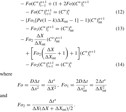
Therefore, the eqs. (5), (6) and (9) in dimensionless form can be given as
FoðCÞniþ11þ ð1þ2FoÞðCÞniþ1
FoðCÞinþþ11¼ ðCÞni ð12Þ fFo1½Peð1kÞXint1 1gðCÞnintþ1
Fo1ðCÞinþ1¼ ðCÞnint ð13Þ
Fo2
X
Xint ðCÞnintþ1
þ Fo2
X
Xint þ1
þ1
ðCÞniþ1
Fo2ðCÞinþþ11¼ ðCÞni ð14Þ
where
Fo¼Dt
x2 ¼
t
X2; Fo1¼
2Dt
x2 int
¼ 2t
X2 int
and
Fo2 ¼
t
XðXþXintÞ=2 :
4. Results and Discussions
In the paper, the method of grid node increasing at the
solid/liquid interface is proposed to deal with the problem of the solute release at the interface during the directional solidification process. The results of the proposed method will be compared with those of other fixed grid methods. The test case for these comparisons is that Pe is set to be 50.
4.1 Fixed grid method with the linear and exponential
extrapolations of the interface concentration
For handling of the solute release at the solid/liquid interface in the one-dimensional mass transfer problem described above, the linear and exponential extrapolation methods are utilized to calculate the interface concentration in a fixed grid system. For example, in Fig. 2,CiandCiþ1can
[image:3.595.69.273.74.307.2]be used to linearly or exponentially extrapolate the interfacial concentration,Cint. The exponential interpolation method is taken from reference.11)The primary difference between the extrapolation methods and the proposed one of adding an extra nodes at the solid/liquid interface is that in extrap-olation methods the interface concentrationCintis calculated or extrapolated by using the concentrations of the nodes nearby. In the proposed method, the interface concentrations of the extra nodes are regarded as unknowns or degrees of freedom in solving the algebraic equations of concentration formulated by the finite difference scheme.
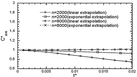
Figure 3 shows the solid concentration distributions for these two methods with the node numbers of 2000 and 8000. The solid concentration CS is equal to the interfacial liquid concentration multiplied by the equilibrium distribution coefficient k. The solid concentration distribution after solidification can be divided into three regions, the initial transient, the steady-state and the final transient regions.18)In the steady-state region, the solid concentration is equal to the initial or averaged concentrationC0, i.e.CS¼1.18)In Fig. 3, the steady value of 8000 nodes is close to one, but the value of 2000 nodes is significantly lower than one, especially for the linear interpolation method. Figure 4 illustrates the averaged concentration varying with time. The averaged values of 8000 nodes are close to one, but the values of 2000 nodes become farther from one as time goes. In these two figures, the solutions of these two methods for 8000 nodes are very similar to each other, but the solutions of the exponential extrapolation method for 2000 nodes are better than those of the linear one.
Fig. 3 Solid concentration distributions of 2000 and 8000 grid points for the fixed grid methods with the linear and exponential extrapolations of the interfacial concentration.
∆x
i
C Ci+1 Ci+2
int
C
int
x ∆
int 2 x ∆
3
i
C+
Control volume of node int (a)
J1 J2
i-1 int i i+1 i+2 i+3
i
C Ci+1 Ci+2
int
C Ci+3
int (∆x ∆x)/ 2
Control volume of node i
(b) +
i-1 int i i+1 i+2 i+3
3
J J4
[image:3.595.312.543.75.204.2] [image:3.595.47.294.518.737.2]4.2 Fixed grid method with extra nodes adding at the solid/liquid interface
This method is an improved method of the extrapolation schemes stated above. Figure 5 shows the solid concentration distributions for this method with the node numbers of 2000 and 8000. In the figure, the concentration distribution of 2000 nodes is nearly the same as that of 8000 nodes and their steady values are close to one. Figure 6 illustrates the averaged concentration varying with time. The averaged values of 8000 nodes are almost equal to one, but the values of 2000 nodes are a little bit higher than one. In the comparisons of the solid concentration and the average concentration distributions from Fig. 3 to Fig. 6, it can be found that the proposed method is better than the linear or exponential extrapolation method stated above.
[image:4.595.54.284.71.201.2]Except the comparisons above, the other computing results are further compared with those taken from the literature. Figure 7 shows the concentration distributions of the 2000th, 6000th and 10000th time steps. In the figure, the variation tendency of the concentration field is the same as that of reference,19) which is shown in Fig. 8. At the solid/liquid interface, the concentration is discontinuous and has a significant concentration difference. Since the liquid solu-bility is higher than the solid one, the redundant solute diffuses into the liquid and makes the solute piled up at the interface.
According to the solution of Clyne and Kurz, the length of the initial transient region is 4D/(Vk),19)i.e. whenx= 4D/ (Vk),C
S ¼1:0. From the computing solution of the proposed
method,CS¼1:007957at this position and the relative error is about 0.79%. Furthermore, Tiller et al.20) and Smith et al.21)had derived the expressions of the solid concentration in the initial transient region:
(i) Tiller solution
Cs¼
C0
k 1 ð1kÞexp kxV
D
ð15Þ
(ii) Smith solution
CS¼
C0
2 (
1þerf
ffiffiffiffiffiffiffi
Vx
4D
r !
þ ð2k1Þexp kð1kÞVx
D
erfc ð2k1Þ
2
ffiffiffiffiffiffi
Vx D
r
" #)
ð16Þ
Fig. 4 Averaged concentration distribution of the whole domain for the fixed grid methods with the linear and exponential extrapolations of the interfacial concentration.
0 0.5 1 1.5 2 2.5 3
0 0.2 0.4 0.6 0.8 1
n=2000 (proposed method) n=8000 (proposed method)
Cs*
X
Fig. 5 Solid concentration distributions of 2000 and 8000 nodes for the fixed grid method with extra nodes adding at the solid/liquid interface.
0.8 1 1.2 1.4 1.6 1.8 2
0 0.005 0.01 0.015 0.02
n=2000 (proposed method) n=8000 (proposed method)
C*
ave
t*
Fig. 6 Averaged concentration distribution of the whole domain for the fixed grid methods with extra nodes adding at the solid/liquid interface.
0 2 4 6 8 10 12 14
0 0.2 0.4 0.6 0.8 1
time steps=2000 time steps=6000 time steps=10000
C*
X
Fig. 7 Concentration distributions at 2000th, 6000th and 10000th time steps for the fixed grid methods with extra nodes adding at the solid/liquid interface.
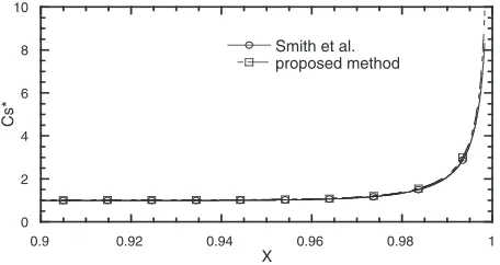
[image:4.595.314.540.72.198.2] [image:4.595.316.542.243.364.2] [image:4.595.53.285.264.393.2] [image:4.595.320.533.422.537.2] [image:4.595.305.550.652.775.2]Figure 9 illustrates the solid concentration distributions in the initial transient region of the proposed method and Tiller and Smith solutions. In the figure, it can be found that these three distributions are very close to each other. Except the solution in the initial transient region, Smith et al. also derived the expression of the solid concentration in the final transient region,21)which is
Cs¼1þ31k 1þkexp
2VðLxÞ
D
þ5ð1kÞð2kÞ
ð1þkÞð2þkÞexp
6VðLxÞ
D
þ. . .þ ð2nþ1Þð1kÞ. . .ðnkÞ ð1þkÞ. . .ðnþkÞ
exp nðnþ1ÞVðLxÞ
D
[image:5.595.58.284.76.201.2]
ð17Þ
Figure 10 illustrates the solid concentration distributions in the final transient region of the proposed method and Smith solution. In the figure, it can be found that the computed distribution agrees fairly well with that of Smith.
From the results shown above, the proposed method can work pretty well for the one-dimensional mass transfer model of the solidification problem. Finally, the proposed method was applied to solve the concentration field of the crystal growth of GaAs (Gallium Arsenide) in a Bridgman fur-nace,22) whose physical model and coordinate system are shown in Fig. 11. In the figure,H,r0andriare the height and the outer and inner radii of the ampoule, respectively.Tmis the melting temperature of GaAs and Tf is the furnace temperature. For establishing the mathematical model, the basic assumptions are (1) the Boussinesq approximation is
used, (2) the fluid flow is laminar and incompressible, (3) the diffusion of dopant in solid is ignored. Based on the assumptions, the governing equations can be written as
1
r
@ðruÞ
@r þ
@v
@z ¼0 ð18Þ
@v
@t þ
1
r
@ðruvÞ
@r þ
@ðvvÞ
@z
¼ 1
@p
@z þ
1
r
@ @r r
@v
@r
þ@ 2v
@z2
gðTTrefÞ ð19Þ
@u
@t þ
1
r
@ðruuÞ
@r þ
@ðuvÞ
@z
¼ 1
@p
@r þ
1
r
@ @r r
@u
@r
u
r2þ
@2u
@z2
ð20Þ
C p @T
@t þ
@ðruTÞ
@r þ
@ðvTÞ
@z
¼1
r
@ @r krr
@T
@r
þ @
@z kz
@T
@z
ð21Þ
@C
@t þ
1
r
@ðruCÞ
@r þ
@ðvCÞ
@z ¼D
1
r
@
@r r
@C
@r
þ@ 2C
@2z
ð22Þ
whereuandvare the velocity components in the radial and axial directions, respectively. p is the pressure, T is the temperature and C is the liquid concentration. is the density,vis the kinematic viscosity,C pis the specific heat and D is the liquid diffusivity. g is the gravitational acceleration, is the coefficient of thermal expansion and
Tref is the reference temperature. kr and kz are the thermal conductivities in the radial and axial directions, respectively. In the beginning of crystal growth, the furnace wall is heated up to a fixed-linear temperature distribution for a certain period of time and then is cooled down to make the crystal grow. Accordingly, the initial conditions of this model are assumed to be the steady solutions in the condition that the furnace wall is set at the first fixed-linear temperature distribution. The temperature distribution of furnace wallTf (along the z direction) at any moment is linear, and decreases 0
0.5 1 1.5 2
0 0.1 0.2 0.3 0.4 0.5 0.6 0.7 0.8
Smith et al. Tiller et al. proposed method
Cs*
X
Fig. 9 Solid concentration distributions in the initial transient region.
0 2 4 6 8 10
0.9 0.92 0.94 0.96 0.98 1
Smith et al. proposed method
Cs*
[image:5.595.56.284.245.366.2]X
Fig. 10 Solid concentration distributions in the final transient region.
ro ri Melt Crystal H t=0 t+dt z z
Furnace wall Ampoule
Tf Tm
[image:5.595.307.551.375.589.2]r TH
[image:5.595.71.262.496.605.2]with time at a constant speed. The expression ofTf can be written as
Tf ¼TH0þGðVgtþzÞ ð23Þ whereGis the temperature gradient of furnace wall and is negative,Vg is called the cooling speed of furnace wall and
TH0 is the highest temperature of furnace wall during the crystal growth.
The boundary conditions of this model can be described as follows.
(1) Boundary conditions of the flow field
(i) ujwall¼vjwall¼0 ð24Þ (ii) ujint¼vjint¼0 ð25Þ
(iii) ujr¼0¼0 ð26Þ
(iv) @v @r
r¼0
¼0 ð27Þ
where the subscript wall means the ampoule wall and the subscript int represents the liquid/solid interface.
(2) Boundary conditions of the temperature field
(i) @T @r
r¼0
¼0 ð28Þ
(ii) Tjz¼0¼Tfjz¼0 ð29Þ
(iii) Tjz¼H¼Tfjz¼H ð30Þ
(iv) Atr¼r0; an equivalent heat transfer
boundary condition is applied, i.e.;
q¼h1ðTTfÞ ð31Þ whereh1is the equivalent heat transfer coefficient,23,24)r0is
the outer radius of the ampoule.
(3) Boundary conditions of the concentration field
(i) @C @r
r¼0¼0 ð32Þ
(ii) @C @z
z¼0
¼0 ð33Þ
(iii) @C @r
r
¼ri
¼0 ð34Þ
whereriis the inner radius of the ampoule. (iv) At the solid/liquid interface;
DðrCnn^Þ ¼Cintð1k0ÞðVV~nn^Þ ð35Þ where Cint is the liquid concentration at the solid/liquid interface andk0 is equilibrium distribution coefficient.VV~is
the growing velocity of the solid/liquid interface andnn^is the unit normal vector of the interface.
The mathematical model is axial-symmetric and the numerical scheme is the finite different method. The SIMPLEC algorithm25)is used to solve the flow field. The modified effective specific heat method26) is utilized to handle the release of latent heat. In the solidification process, because the solubility of liquid solute is higher than that of solid, the surplus solute will be released from the solid/liquid interface into the liquid, which is the main source of increasing liquid solute. If the effect of solute release is not handled appropriately, the concentration solutions will diverge very easily.
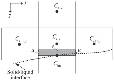
The boundary condition of concentration field at the solid/
liquid interface is given by eq. (35). To deal with the problem of solute release at the solid/liquid interface, extra nodes are added on the interface, as shown in Fig. 12. In the figure,Cint is the extra node. The right hand side of eq. (35) is main source of increasing liquid solute during solidification. Because it is difficult to evaluate the growth velocityVV~, the sweeping volume of the moving interface in a time step is used instead. Accordingly, the increased rate of solute in a time step can be given by
Cintð1k0Þ
8int
t ð36Þ
where 8int is the sweeping volume. By using the control volume method, the difference equation of the extra nodeCint at the interface (Fig. 12) can be written as
Cintnþ1ð1k0Þ8int
t þD Cnþ1
iþ1;jC nþ1 int
r Ae
þDC
nþ1 i;j C
nþ1 int
s AnþD
Cniþ11;jCnintþ1
r Aw
vn
Cin;þj1þCintnþ1
2 Anþue
Cinþþ11þCintnþ1
2 Ae
uw
Cnþ1 i1;jþC
nþ1 int
2 Aw¼
Cnintþ1Cnint
t 8 ð37Þ
where the superscript n represents the index of time step.ue,
Ae,uw,Aw,vnandAnare the velocities and areas of the east, west and north control surfaces, respectively.8is the volume of the control volume andsis the distance from Cni;þj1 to
Cnþ1 int .
Figure 13 shows the computed temperature and flow fields (isotherms and streamlines) of GaAs in the ampoule for two Rayleigh numbers. Raleigh number is defined as
Ra¼ gðGHÞri3=ð‘Þ ð38Þ
where is the coefficient of thermal expansion, is the kinematic viscosity and‘ is the liquid thermal diffusivity.
Rayleigh number for Fig. 13(a) and 13(b) is 100 and the number for Fig. 13(c) and 13(d) is 10000. In the figure, it rotates from the vertical to the horizontal for convenience and the direction of gravity is towards the right. The curved isotherm next to the bottom of streamlines is the solid/liquid interface. The curved interface induces the natural convec-tion, which causes a clockwise circulation in the melt. The
, i
C
i
C−1,
, i
C
1, i
C+
Solid/liquid interface
int
C
e
u
w
u vn
z
r
j−1
j
[image:6.595.328.525.76.217.2]j j
corresponding concentration fields (isoconcentrates) of dop-ant Se in the liquid GaAs are illustrated in Fig. 14.
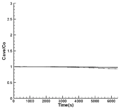
From Fig. 14, it can be found that the higherRahas the stronger flow field, but does not have a significant effect on the temperature field and the shape of solid/liquid interface. The concentration field can be affected by not only diffusion but also convection. Because of the Schmidt number (Sc¼=D) of dopant Se in GaAs is 42, the convective effect is expected to be much larger than the diffusive one. In Fig. 14, the isoconcentrates are significantly distorted by the melt flow, especially in the case of Ra¼10000. With the stronger velocity field resulted from the higherRa, the solute from the interface is taken into the melt faster and therefore the maximum concentration becomes smaller. However, due to the induced circulation, the solute accumulates around the corner between the interface and the central axis, where the concentration field has its maximum value. Finally, Figure 15 illustrates Cave/C0varying with time forRa¼100
and 10000, where Cave and C0 are the averaged and initial
concentrations respectively. In the figure, the thick line is
Ra¼100 and the thin line isRa¼10000. It can be found that the averaged concentrations are very close equal to the initial one.
5. Conclusion
In this paper, extra nodes added on the solid/liquid interface in a fixed grid system are proposed to solve the mass transfer problem in a directional solidification process. A one-dimensional problem is firstly used to test the proposed method. The computing results will be compared with those
of the linear and exponential extrapolation methods and the analytical solutions from the literature. From the compar-isons of the steady value of the solid concentration and the average concentration distributions for the one-dimensional problem, the proposed method is better than the linear or exponential extrapolation method. In the initial and final transient regions of the one-dimensional problem, the computed solid concentrations are very close to those taken from the literature. Finally, The feasibility of the proposed method is further testified by applying it to solve the concentration field of the crystal growth of GaAs in a Bridgman furnace.
(a)
Time = 3200 s, Tmax=1256°C, Tmin=1216°C,∆ T=1.6°C,
Ψmax =0.000452, Ψmin =0, ∆ Ψ=0.00005
g (b)
Time = 6400 s, Tmax=1246°C, Tmin=1206°C,∆T=1.6°C,
Ψmax =0.000454, Ψmin =0, ∆Ψ=0.00005
g
(c)
Time = 3200 s, Tmax=1256°C, Tmin=1216°C,∆T=1.6°C,
Ψmax =0.0439, Ψmin =0,∆Ψ=0.003
g g
(d)
Time = 6400 s, Tmax=1246°C, Tmin=1206°C,∆T=1.6°C,
[image:7.595.92.506.80.340.2]Ψmax =0.0438, Ψmin =0, ∆Ψ=0.003
Fig. 13 Computed temperature and flow fields,Ra¼100for (a)(b) and 10000 for (c)(d).
(a)
Time = 3200 s, Cmax=2.08, Cmin=1.0, ∆C=0.1
g (b)
Time = 6400 s, Cmax=2.83, Cmin=1.0, ∆C=0.1
g
(c)
Time = 3200 s, Cmax=1.202, Cmin=1.0, C=0.01
g (d)
Time = 6400 s, Cmax=2.031, Cmin=1.0, C=0.01
[image:7.595.324.529.415.601.2]g
Fig. 14 Computed liquid concentration field (isoconcentrates),Ra¼100for (a)(b) and 10000 for (c)(d).
Fig. 15 Cave=C0of the whole domain varying with time forRa¼100and
REFERENCES
1) M. Salcudean and Z. Abdullah: Int. J. Numer. Methods Eng.25(1988) 445–473.
2) V. R. Voller and C. R. Swaminathan: Int. J. Numer. Methods Eng.30
(1990) 875–898.
3) H. Hu and S. A. Argyropoulos: Modelling Simul. Mater. Sci. Eng.4
(1996) 371–396.
4) J. Caldwell and Y. Y. Kwan: Commun. Numer. Meth. Eng.20(2004) 535–545.
5) G. Labonia, V. Timchenko, J. E. Simpson, S. V. Garimella, E. Leonardi and G. de Vahl Davis: Numer. Heat Transfer, Part B.34(1998) 121– 138.
6) C. Y. Li, S. V. Garimella and J. E. Simpson: Numer. Heat Transfer, Part B.43(2003) 117–141.
7) H. Zhang, V. Prasad and M. K. Moallemi: Numer. Heat Transfer, Part B.29(1996) 399–421.
8) R. W. Lewis and K. Ravindran: Int. J. Numer. Meth. Eng.47(2000) 29–59.
9) S. C. Gupta: Comput. Methods Appl. Mech. Eng.189(2000) 525–544. 10) V. R. Voller, A. D. Brent and C. Prakash: Int. J. Heat Mass Transfer32
(1989) 1719–1731.
11) V. Timchenko, P. Y. P. Chen, E. Leonardi, G. de Vahl Davis and R. Abbaschian: Int. J. Heat Mass Transfer43(2000) 963–980.
12) C. W. Lan and F. C. Chen: Comput. Methods Appl. Mech. Eng.131
(1996) 191–207.
13) P. M. Adornato and R. A. Brown: J. Cryst. Growth80(1987) 155–190. 14) S. Brandon and J. J. Derby: J. Cryst. Growth121(1992) 473–494. 15) C. Stelian, J. L. Plaza, F. Barvinschi, T. Duffer, J. L. Santailler, E.
Dieguez and I. Nicoara: Cryst. Res. Technol.36(2001) 651–661. 16) C. Stelian, T. Duffer and I. Nicoara: J. Cryst. Growth255(2003) 40–51. 17) C. Barat, Ph.D. Thesis, University of Rennes, 1995.
18) M. C. Flemings:Solidification processing, (McGraw-Hill, New York, USA 1974) pp. 31–57.
19) W. Kurz and D. J. Fisher: Fundamentals of solidification, 4th ed., (Trans tech publication Ltd, Switzerland 1998) pp. 117–132. 20) W. A. Tiller, K. A. Jackson, J. W. Rutter and B. Chalmers: Acta
Metallurgica1(1953) 428–437.
21) V. G. Smith, W. A. Tiller and J. W. Rutter: Can. J. Phys.33(1955) 723–745.
22) J. A. Kafalas and A. H. Bellows: NASA Technical Memorandum1
(1988) 337–347.
23) D. H. Kim, PhD Thesis, MIT, 1990.
24) D. H. Kim and R. A. Brown: J. Cryst. Growth109(1991) 66–74. 25) J. P. Van Doormaal and G. D. Raithby: Numer. Heat Transfer7(1984)
147–163.