Criterion for Constitutional Supercooling at Solid Liquid Interface in Initial Transient Solidification with Varying Solute Content at Interface

Criterion for Constitutional Supercooling at Solid-Liquid Interface

in Initial Transient Solidification with Varying Solute Content at Interface

Hiroshi Kato and Yukihiko Ando

Division of Mechanical Science and Engineering, Graduate School of Science and Engineering, Saitama University, Saitama 338-8570, Japan

A criterion for appearance of the constitutional supercooling at the solid-liquid interface in the initial transient solidification is discussed theoretically and experimentally. First, a relation between the moving velocity of the interface and the solute content was analyzed to derive a moving velocity of the interface under a simple model of the linear change in the solute content at the interface. And, a criterion for appearance of the constitutional supercooling at the planar interface was analyzed to obtain the distance of the stable growth of the interface with the planar shape. Then, the solidification experiment was carried out with the Al-4 mass% Cu alloy: the aluminum alloy was inserted in the alumina tube of 0.4 to 2 mm in inner diameter and heated for2:54h under a temperature gradient to obtain the stationary interface, and then the alumina tube was cooled in the furnace for 0 to 45 s. After furnace cooling, the alumina tube was quenched in water to observe the interface. The interface with the planar shape appeared for2030s after the start of furnace cooling, and then the columnar structure grew ahead of the interface. Then the solute content in the solid behind the interface was analyzed to show that the solute content in the specimen quenched after furnace cooling was different from that in the specimen quenched without furnace cooling. The experimental results were compared with the theoretical calculations to infer that the interface moved with the planar shape for a short time after the start of furnace cooling, and then the interface became unstable to form the columnar structure. [doi:10.2320/matertrans.M2010253]

(Received July 27, 2010; Accepted November 10, 2010; Published December 22, 2010)

Keywords: solidification, solid-liquid interface, initial transient, aluminum alloy, morphological stability

1. Introduction

There are increasing attention to micro-machines and micro-devices, which accelerated development of production techniques of micro-components, such as lithography, rapid prototyping, and so on. In the casting field, also, there have been many reports1–5) _{on micro-casting techniques and} production of micro-mold, but there are no reports on formation mechanisms of the solidification structure. In the solidification of micro-scale components, the steady state solidification is very limited or does not exist, but the initial and terminal transient solidifications are dominant. There-fore, it is very important to realize the solidification process in the transient solidification, especially in the initial transient solidification, in order to understand the solidification structure in the micro-components.

On the solute redistribution in the initial transient solid-ification, there are many reports, such as the approximate analysis by Tiller et al.,6) and the rigorous analyses by Smith7) and by Nastac.8) These analyses have been carried out under the constant moving velocity of the solid-liquid interface. Kato,9)_{however, has pointed out that in the initial} transient solidification, the solute content at the interface changes with the movement of the interface resulting in the change in the interfacial temperature, which means even though the cooling velocity and the temperature gradient are constant, the moving velocity of the interface changes in the initial transient solidification. Then he derived a relation between the moving velocity of the interfaceRand the solute content in the liquid at the interface Ci

L, by equating the temperature distributions in the liquid ahead of the interface described by the fixed coordinate system and the moving coordinate system with the interface as follows,

R¼R0

mL

GL

dCi

L

dt ; ð1Þ

where R0 is the nominal moving velocity of the interface

defined by the cooling velocityV0divided by the temperature

gradientGL, andmLis the gradient of the liquidus line. Huang

et al.10)_{obtained the length of the initial transient region by} using the eq. (1). In these reports, it can be said that the dif-ferent moving velocity of the interface may largely influence the solute redistribution in the initial transient solidification. Also there have been many reports on the morphological stability of the solid-liquid interface. On the steady state solidification process, analyses have been reported based on the constitutional supercooling by Tiller et al.6)_{and on the} perturbation of the interface by Sekerka et al.,11–13) _by Voronkov,14) _{by Delves.}15,16) _{Also, Nastac}8) _{reported the} morphological stability of the interface in the initial transient solidification. These analyses have been conducted under constant velocity of the interface, but as mentioned above, the moving velocity of the interface is different from the nominal velocity in the initial transient solidification, which results in different solute redistributions from that of the nominal moving velocity. Recently Yao et al.17)_discussed the nucleation in the initial transient solidification in consideration of the change in the solute content by using the eq. (1), but they did not discuss the criterion for the morphological stability in the initial transient solidification.

In the present work, a moving velocity of the interface was derived in the initial transient solidification, and then the criterion for appearance of the constitutional supercooling at the interface was discussed to obtain a distance of the stable growth of the planar interface. Then, the solidification experiment was carried out by using the Al-4 mass% Cu alloy to observe the solidification structure, and the solute content profile was analyzed in the solid around the interface. Finally, the experimental results were compared with the *_{Graduate Student, Saitama University. Present address: Calsonic Kansei}

theoretical calculation to discuss the stable movement of the interface in the initial transient solidification.

2. Mathematical Analysis

2.1 Relationship between moving velocity of interface and solute content in initial transient solidification In this section, the movement of the planar interface is analyzed in the initial transient solidification of a binary alloy with a solute content ofC0and a partition coefficient ofk. In

the present discussion, the partition coefficientkis assumed to be constant and less than unity. Symbols used in the present paper are summarized in Appendix.

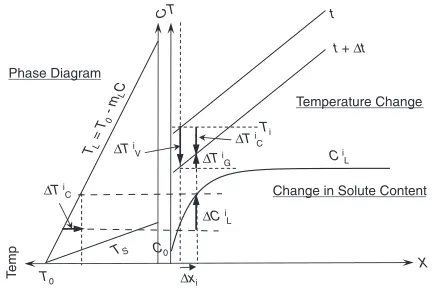
At the beginning of the solidification, the solid with the solute content ofkC0appears neighboring the liquid ofCoto form the solid-liquid interface. When the time passes fromt to tþt and the interface moves from a position xi to xiþxi, as shown in Fig. 1, the interfacial temperature decreases byTi

Vdue to cooling, and increases byTGi due to movement of the interface, which are given by

T_Vi ¼ ViðtÞt; ð2Þ

T_Gi ¼GiðtÞxi; ð3Þ

where Vi_{ðtÞ and G}i_{ðtÞ are the cooling velocity and the} temperature gradient in the liquid ahead of the interface at time t, respectively. Also, the interfacial temperature de-creases byT_Ci with increasing solute content in the liquid at the interfaceC_Li as follows,

T_Ci ¼ mLCiLðtÞ; ð4Þ

where mL is the gradient of the liquidus line in the phase diagram, and is taken to be positive. These temperature changes should be balanced to give the following relation,

T_Vi þT_Gi ¼ T_Ci: ð5Þ

)ViðtÞtþGiðtÞxi¼ mLCLiðtÞ: ð6Þ

When the moving velocity of the interface ðdxi=dtÞ is represented byRðtÞ, eq. (6) is rewritten as follows,

RðtÞ ¼dxi

dt ¼

1

Gi_ðtÞ V

i ðtÞ mL

dCi_L

dt

: ð7Þ

When the cooling velocity and the temperature gradient are constant and represented byV0andGL, respectively, eq. (7)

is rewritten as follows,

RðtÞ ¼R0

mL

GL

dCi_L

dt ; ð8Þ

where R0 is the nominal moving velocity of the interface

given byV0=GL. Equation (8) is the same as eq. (8)–(10) in the ref. 9). Since the moving velocity RðtÞtakes a positive value, the right side of eq. (8) should be positive to give the following relation,

dCi

L

dt

R0GL

mL

: ð9Þ

By integrating eq. (9) in consideration of the condition: at

t¼0,C_Li ¼C0,

Ci_LR0GL

mL

tþC0: ð10Þ

This equation gives the upper limit of the solute content in the liquid at the interface at time t in the initial transient solidification.

In the present paper, the discussion is limited in the initial transient solidification, but eqs. (7) and (8) are also appli-cable to the unsteady solidification, such as the terminal transient solidification.

2.2 Moving velocity of interface in initial transient solidification

In this section, a very short time after the start of solidification is considered, and it is assumed that the cooling velocity and the temperature gradient are constant to be V0

andGL, respectively. Also, in the preceding section, it was shown that there is the upper limit in the changing rate of the solute content at the interface, and hence it is assumed that the solute content Ci

L in the liquid at the interface linearly increases with time as follows,

Ci_L¼KLtþC0; ð11Þ

where KL is the proportional constant. In this case, the interface moves with a constant velocityR _{given by}

R¼R0

mL

GL

KL: ð12Þ

And, when the planar interface stably moves, the solute content C_Si in the solid at the interface changes with the following rate,

dCi_S

dx ¼

kGL

mL

R0R

R

: ð13Þ

When the interface moves with a constant velocity, the solute content in the initial transient solidification is given by Tilleret al.6)_{and by Smithet al.,}7)_{and it is known that in the} early stage of the solidification, the solute content given by Tiller et al.6) _{shows the similar change to the rigorous} solution given by Smith et al.7) _{Therefore, the present} analysis was carried out by using the solution by Tiller

et al.,6)and the solute content in the liquid is given by

CL¼C0

1k

k 1exp k

ðRÞ2

DL

t

exp R

DL

ðxRtÞ

þ1

: ð14Þ

X Ci

L

Te

m

p TS

TL

=T

0

-m

L

C

t

t+∆t T

∆Ti V

Ti

∆xi

∆Ci L

∆Ti G

∆Ti C

Temperature Change

Change in Solute Content Phase Diagram

C

∆Ti C

T0

C0

The solute content in the liquid at the interface is obtained by inserting x¼Rt in the above equation, and then differ-entiated by time to obtain the changing rate of the solute content. Finally, by insertingt¼0, the changing rate of the solute content in the liquid at the interface is obtained in a very short time after the start of solidification, and is given by

@Ci L

@t _t¼0 ¼

C0ð1kÞ

DL

ðRÞ2: ð15Þ

By substituting eq. (15) into eq. (8), the following quadratic equation concerning toR _{is obtained,}

mLC0ð1kÞ

DLGL

ðRÞ2þRR0 ¼0: ð16Þ

The positive solution of this equation is given by,

R ¼R0

2

1þ

ffiffiffiffiffiffiffiffiffiffiffiffiffiffiffiffiffiffiffiffiffiffiffiffiffiffiffiffiffiffiffiffiffiffiffiffiffiffiffiffiffiffiffi 1þ4mLC0ð1kÞ

DL

R0

GL

s

¼R0

2

1þ

ffiffiffiffiffiffiffiffiffiffiffiffi

1þ

s ; ð17aÞ

where

¼4mLC0ð1kÞ

DL

¼4k ; ¼GL

R0

: ð17bÞ

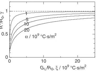
The parameterð¼ ðmLC0=DLÞð1kÞ=kÞis the criterion for the constitutional supercooling given by Tiller et al.6) As shown in Fig. 2, the moving velocity of the interface R monotonically increases with increasingGL=R0from zero to

approach the nominal moving velocityR0.

2.3 Criterion for stable growth of planar interface in initial transient solidification

In this section, the criterion for the stable growth of the planar interface in the initial transient solidification is discussed following the criterion of the constitutional super-cooling. The temperature distribution in the liquid ahead of the interface expected from the solute distribution6)is given by

TL¼T0mLC0

1k

k 1exp k

ðRÞ2

DL

t

exp R

DL

ðxRtÞ

þ1

: ð18Þ

From the above equation, the temperature gradient in the liquid ahead of the interface is calculated. Then by comparing with the real temperature gradient GL, the criterion for the stability of the planar interface is obtained as follows,

mLC0

1k k

R

DL

1exp kðR _Þ2

DL

t

GL; ð19Þ

wheret_{is the time while the planar interface stably moves,} and eq. (19) is changed as follows,

t_¼1

k

DL

ðR_Þ2

ln 1 DL

mLC0

k

1k

GL R : ð20Þ

In eq. (20), the logarithmic term should be positive to give the following restriction.

GL

R <

mLC0

DL

1k k

¼ : ð21Þ

Under this restriction, the distance x _{(¼Rt) while the} planar interface stably moves is obtained from eq. (20) as follows,

x¼1

k

DL

R

ln 1 DL

mLC0

k

1k

GL R : ð22Þ

After substitution ofR_{, eq. (22) is changed as follows,}

¼ kR0

DL

x

¼ 1

2 1þ

ffiffiffiffiffiffiffiffiffiffiffiffi

1þ

r

ln 1 1þ

ffiffiffiffiffiffiffiffiffiffiffiffi 1þ r ; ð23aÞ

where_{is the normalized distance ofx, and}

¼ DL 2mLC0

k

1k

¼2k

¼

1

2 : ð23bÞ

The normalized distance _{of the stable growth} monotoni-cally increases with increasing GL=R0 to infinity at

=ðkþ1Þ, as shown in Fig. 3 by using k of 0.14. In the figure, however, the larger value of the distance_{is not valid} because the model is applicable only for the early stage of the solidification. In the present calculation, the changing rate of the solute content was derived att¼0. Here, the maximum distanceXcis defined as the distance at which the changing rate of the solute content decreases byexpð"Þof the initial value, where 0< " <1, and is obtained from eq. (14) as follows,

X_c ¼ DL

2kR0

1þ ffiffiffiffiffiffiffiffiffiffiffiffi 1þ r "; ð24Þ or normalized,

_c ¼ kR0

DL

X_c ¼1

2 1þ

ffiffiffiffiffiffiffiffiffiffiffiffi 1þ r ": ð25Þ

The normalized maximum distancecfor"¼1is included in Fig. 3. In the figure, c is decreased with increasing GL=R0 to converge unity, and the normalized distance of

the stable growth represented by a dashed line exceedsc, and hence is not valid.

Additionally, when the interface moves with the nominal moving velocityR0, there is a region of the stable growth of

0 10 20

0 0.5 1

GL/R0, ξ / 109 °C·s/m2

R

*/

R0

,

γ

α / 109 °C·s/m2

1

10 20 5

Fig. 2 Change inR_=R

the planar interface because the pile up of the solute is so small in the beginning of the solidification. In this case, the distancexnomwhile the interface stably moves is given by,

xnom¼

1

k

DL

R0

ln 1 DL

mLC0

k

1k

_G

L

R0

: ð26Þ

or normalized,

nom¼ k

R0

DL

xnom¼ log 1

: ð27Þ

3. Experimental Procedure

3.1 Preparation of specimen

Slender alumina tubes containing the Al-4 mass% Cu alloy were prepared for the solidification experiment. First, the aluminum alloy was melted in the carbon crucible in the electric furnace heated at 800_{C. Then the alumina tube was} inserted in the molten alloy from the top of the electric furnace, kept for a few minute for preheating, and then the molten alloy was sucked into the tube by a slight vacuum. Then the alumina tube containing the molten alloy was cooled to room temperature, and was cut into pieces of 150200mm in length for the solidification experiment. In the present work, alumina tubes of three sizes (inner

diameterthickness = 2 mm1 mm, 1 mm0.5 mm,

0.4 mm0.3 mm) were used.

3.2 Solidification experiment

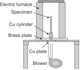
The solidification experiment was carried out with a setup schematically shown in Fig. 4, as follows,

(1) The alumina tube was inserted in a copper cylinder placed on a copper plate situated below the electric tubular furnace.

(2) The furnace was heated up to and kept at 800_{C for} 2:54h, during which the copper plate was cooled by air with a blower.

By the preliminary experiment, it was found that the amount of the liquid droplet was decreased in the solid behind the interface with increasing heating time, and after heating of alumina tubes with a inner diameter of 0.4 mm and 2 mm for 2.50 h and 4 h, respectively,

almost all of the liquid droplets disappeared in the solid and the interface became planar. At this time, the interface situated at a fixed position with a planar shape, and hereafter referred to as the stationary interface. (3) After heating for the required time to obtain the

stationary interface, the electric source was switched off to cool the furnace.

(4) After cooling for required times (045s), the alumina tube was quenched in water by removing the cupper plate.

Then the alumina tube was sectioned, mounted, polished and etched with a water solution of sodium hydroxide for observation of the microstructure.

The temperature measurement was also carried out with alumina tubes with an inner diameter of 1 mm and 2 mm: shallow slits are made on the alumina tube at 50 mm, 60 mm, 70 mm, 80 mm from the bottom of the tube to expose a part of the aluminum alloy, and the K thermocouples of 0.3 mm in diameter were fixed with heat-resistant cement. However, the temperature measurement of the alumina tube with an inner diameter of 0.4 mm was not conducted because of the difficulty of setting the thermocouple.

3.3 Metallography and chemical analysis

The microstructure near the interface was observed by using the optical microscope. Then the solute profile in the solid around the interface was analyzed by using the electron probe X-ray micro-analyzer (EPMA) with the acceleration voltage of 15 kV and the sample current of 0.5 nA. The analysis was carried out along the longitudinal direction of the alumina tube from the planar interface to a position in the solid 300mm apart from the interface with an interval of 1mm, and then the data were averaged at every ten points to reduce scatter of data.

4. Results and Discussion

4.1 Microstructure at interface

Solid-liquid interfaces in the alloy specimen quenched after heating for2:54h are shown in Fig. 5, in which the interface with a planar shape was observed. In the present work, the solid-liquid interfaces under different situations are discussed. In the preceding section, the interface situated at a fixed position under the steady temperature profile was defined as ‘‘the stationary interface’’. And, in Fig. 5, the interface was observed in the specimen after quenching, but

Cu plate Specimen Electric furnace

Cu cylinder

Brass plate

Blower

Fig. 4 Setup for unidirectional solidification.

10 20 30

0 2 4 6 8

GL/R0, ξ / 109 °Cs/m2

Normalized distance

α / 109 °Cs/m2

1 5 10 20

∆c* (ε = 1)

20

1

δ* 2

Fig. 3 Changes in normalized distance_{and maximum distance}

cfor

might be different from one before quenching. Therefore, this interface is called as ‘‘the observed interface’’. Finally, the interface existed or moving in the specimen before quenching is called as ‘‘the interface’’.

In Fig. 6, temperature changes during the furnace cooling of the specimen with a diameter of 1 mm are shown. Assuming that the initial interfacial temperature was coin-cident with the liquidus temperature (647C) of the Al-4 mass% Cu alloy,18)the position of the stationary interface

was estimated to be 60mm70mm from the specimen

bottom. The specimen of 2 mm in diameter also showed the same temperature change, but took slightly lower temper-atures than those in the specimen of 1 mm in diameter.

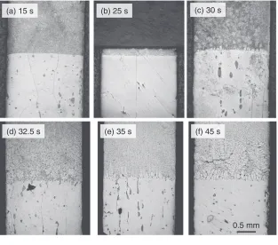
Figures 7–9 show microstructures in the specimen quenched after furnace cooling of different times. In a short time after the start of furnace cooling, the interface of the planar shape was observed. After 2030s, the cellular or columnar structure appeared on the observed interface. With the passage of the time, the columnar structure developed and changed into the dendrite with side arms. In addition, in Fig. 7(b), the specimen was broken just above the observed interface, and in the other specimens, cracks appeared above the observed interface, which are caused by sudden shrinkage of the specimen during quenching. Figure 10 shows changes

in the length of the columnar structure with the elapsed time after the start of furnace cooling. In the figure, the columnar structure shows a finite length in a short time after the start of furnace cooling. This is because the length of fine structures appeared on the interface was included in the length of the columnar structure. The fine structure was observed on the interface in all specimens quenched with/without the furnace cooling, and hence it was thought to be formed during quenching. Therefore, it was thought that the columnar structure appeared when the coarser structure than the fine structure was observed on the interface, namely2030s after the start of furnace cooling, and then grew with a consid-erable rate. In the figure, dashed lines are the estimated lengths of the structure being assumed to develop with the nominal growth velocity R0, and gradients of the estimated

length show a good agreement with those of the experimental results except the initial stage.

To verify the relation between the delay time before appearance of the columnar structure and the specimen diameter, the temperature change was precisely examined just after the start of furnace cooling. Figure 11 shows the temperature change after the start of furnace cooling at a position where the stationary interface might situated (here-after referred to as the initial interface position). Although the temperature was not measured at the initial interface position, the temperature at each position decreased with the same rate as shown in Fig. 6, and hence the temperature change at the initial interface position was estimated by interpolating those obtained by thermocouples situated just below and above the initial interface position. Although the delay time before the appearance of the columnar structure was different for two specimens, the temperature at which the columnar structure appeared was almost the same, and it was thought that the difference in the delay time was mainly due to difference in the cooling velocity.

Next discussion is on the considerably long delay time before appearance of the columnar structure. As shown in Fig. 11, the temperature was almost constant for a while and then decreased. Therefore it might be thought that the columnar structure appeared when the temperature drop

0.5 mm

Solid

Liquid

(a) d : 2 mm

(b) d : 1 mm

(c) d : 0.4 mm

0 100 200 300 400

400 500 600 700

800 _{Liquidus temp.}

Elapsed time, t / s

T

e

mperature,

T

/ °C

Position, h (mm)

50 60 70 80 F.T.

Fig. 6 Change in temperatures at different positions in specimen of 1 mm diameter during furnace cooling. F.T. means a temperature of atmosphere in the furnace.

started. However, the delay time was not coincident with the stationary time while the temperature was almost constant, but the columnar structure appeared several seconds after the start of temperature drop. As the reason of this discrepancy, following phenomena may be pointed out:

(1) A supercooling occurred following the rapid cooling to give the driving force for forming the columnar structure.

(2) The interface stably moved with the planar shape, and then became unstable to form the columnar structure.

Mizukami et al.19–21) _{studied the initial solidification} process of 18 mass% Cr-8 mass% Ni stainless steel quenched on a copper substrate, and reported that a large supercooling occurred on the specimen surface before the start of solid-ification, and then the cellular structure was formed on the substrate. In the present work, however, the solidification started from the stationary interface with a relatively slow rate, and no need of a large supercooling for the start of solidification. Also, even if the supercooling occurred, there was only a small difference in the specimens quenched

(a) 15 s (c) 30 s

(d) 32.5 s (e) 35 s (f) 45 s

0.5 mm (b) 25 s

Fig. 7 Change in solid-liquid interface in specimens of 2 mm in diameter with elapsed time.

(d) 25 s

(a) 15 s (b) 20 s (c) 22.5 s

(e) 27.5 s

0.5 mm (f) 30 s

with/without the furnace cooling. Therefore, in the case (1), the furnace cooling did not considerably affect the solute redistribution in the solid behind the interface. To the contrary, when the interface stably moved with the planar shape before the columnar structure appeared as the case (2), the solute concentration gradually increased from the initial content before quenching in water. In this case, existence/ absence of the furnace cooling before quenching might affect the solute profile in the solid behind the interface.

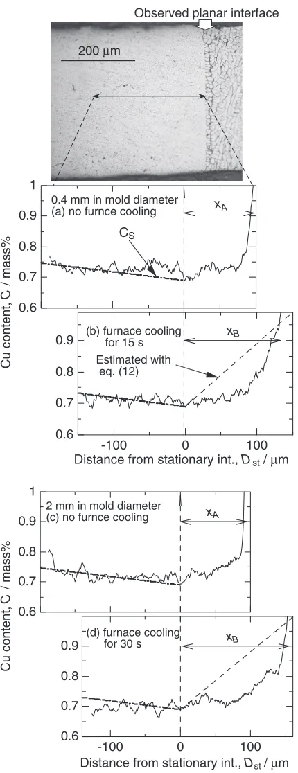
To specify the reason of the delayed appearance of the columnar structure, the solute profile in the solid behind the observed interface, namely in the lower region below the observed interface, was analyzed. Figure 12 compares the solute distributions behind the observed interface in the specimen quenched without the furnace cooling (hereafter referred to as the specimen-NF) and one quenched after the furnace cooling (the specimen-F). The optical micrograph at the interface was also included in the figure. As shown in the

micrograph, the right side of the figure was coincident with the fine structure appeared on the observed interface, and the steep increment of the solute content a few mmbefore the right side of the profile is due to the second phase Al2Cu in

the fine structure.

In the present work, the solidification started from the stationary interface, and as schematically shown in Fig. 13, there was a solute distribution following the solidus line in the solid behind the stationary interface,18) _{and with the} movement of the interface, the solute content increased in the liquid at the interface. Following this situation, the position of the stationary interface was fixed as follows. First, the solidus line was plotted to fit the solute profile in the solid apart from the observed interface as shown by dashed-dotted lines in Fig. 12. Then the stationary interface was fixed at a position where the line crosses the solute profile. Following this procedure, the stationary interface was assumed to be at a position 100150mm behind the observed interface.

10 s 15 s 20 s

25 s 30 s 45 s

0.1mm

10 20 30 40 50

0.5 1 1.5 2 2.5

0

Elapsed time, t / s

L. columnar struct.,

Lcolum

/ mm

Exp R0 Diameter

0.4 mm 1 mm 2 mm

Fig. 10 Change in length of columnar structuresLcolumwith elapsed time

of furnace cooling.

0 10 20 30 40 50

630 640 650

0 0.5 1 1.5

Elapsed time, t / s

T

e

mperature,

T

/ °C

Lcolum

(mm)

2 mm dia. 1 mm dia.

V0: 0.38 °C/s

V0: 0.53 °C/s

Fig. 11 Change in temperature at position of solid-liquid interface with elapsed time.

The solute distribution from the stationary interface to the observed interface was slightly different for both cases. Even in the specimen-NF, the solute concentration largely de-creased from the observed interface to the minimum solute content. This was thought that during cooling in the quenching, the interface moved keeping the planar shape at some distance to follow the increase of the solute content from the minimum solute content of kC0. On the contrary,

in the specimen-F, during the furnace cooling, the interface

moved with the planar shape with gradually increasing the solute content, and then during quenching, the interface moved additionally at some distance to follow the increase in the solute content. Therefore, the distance xB from the observed interface to the stationary interface in the specimen-F was larger than the distancexAin the specimen-NF.

Dashed lines in the figures are the solute content in the solid ahead of the stationary interface estimated with eq. (13) and will be explained precisely in the next section.

Difference in the solute distributions behind the observed interface supports the case (2), and it was thought that after the start of furnace cooling, the interface stably moved with the planar shape for 2030s, and then the morphological change of the interface occurred into the cellular or columnar structure. In the next section, the experimental results were compared with the theoretical calculations.

4.2 Comparison between experimental results and the-oretical calculations

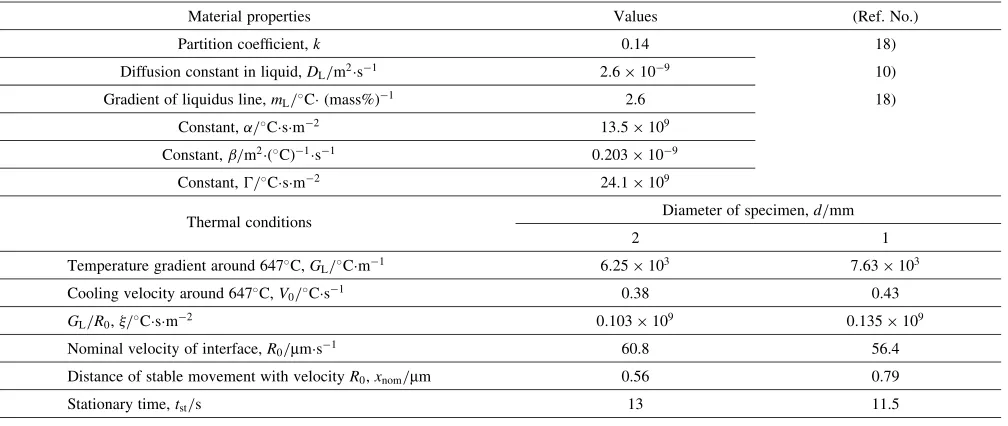
In this section, the solidification parameters, such as the moving velocity of the interface and so on, are calculated with the thermal conditions. In the present experiment, as shown in Fig. 11, just after the start of furnace cooling, the temperature at the interface changed very slowly, and then decreased with a constant cooling velocity. Therefore, the temperature change was approximated by dashed-dotted lines in Fig. 11; the temperature was constant for the stationary time of 13 s and 11.5 s, and then cooled with a constant velocity V0¼0:38C/s and 0.53C/s, for

speci-mens of 2 mm and 1 mm in diameter, respectively.

Then, by using values of material properties and thermal conditions tabulated in Table 1, the solidification parameters, such as the moving velocityR_{, the moving distancex and} the timet_{of the stable movement of the interface, and so on} were calculated as shown in Table 2.

In Table 2, for the specimen of 2 mm in diameter, the moving velocity R _{of 9.64mm/s is far lower than the} nominal growth rate R0¼60:8mm/s, and the moving

distancex _{of 22.4mmis comparable with the difference in} the distance (xBxA) of about 60mmand far longer than the nominal distancexnom¼0:56mm. Moreover, the calculated delay timetdelaybefore appearance of the columnar structure (¼tstþt) was 15.3 s for the specimen of 2 mm in diameter

200 µm

Observed planar interface

0.6 0.7 0.8 0.9 1

Cu content,

C

/ mass%

0.4 mm in mold diameter

(a) no furnce cooling xA

CS

-100 0 100

0.6 0.7 0.8 0.9

Distance from stationary int., Dst / µm (b) furnace cooling

for 15 s

xB

Estimated with eq. (12)

0.6 0.7 0.8 0.9 1

Cu content,

C

/ mass%

2 mm in mold diameter

(c) no furnce cooling xA

-100 0 100

0.6 0.7 0.8 0.9

(d) furnace cooling for 30 s

Distance from stationary int., Dst / µm

xB

Fig. 12 Comparison of copper content profiles in specimens of 0.4 mm in mold diameter (a) and (b), and 2 mm in mold diameter (c) and (d) with/ without furnace cooling.

Distance Ci

L

C0

C

kC0 CS

Stationary interface

Solid Liquid Moving of interface

and was longer than the delay time tdelay of 13.9 s for the specimen of 1 mm in diameter, and this magnitude relation was consistent with that of the experimental delay time.

Finally, the changing rate (dCi_s=dx) of the solute content in the solid at the interface following the movement of the interface was estimated by using eq. (13) to be 0.0018 mass%/mm and 0.0019 mass%/mm for the specimens of 2 mm and 1 mm in diameter, respectively. As shown in Fig. 12, the estimated solute content ahead of the stationary interface (dashed lines in the figures) showed a rather good agreement with the measured solute profile, but was slightly higher than the measured one.

From these discussions, the experimental results were relatively in good agreement with the theoretical calculations carried out with a simple model, and it was inferred that the interface stably moved with the planar shape for a short time in the furnace cooling, and then became unstable to result in the morphological change into the cellular or columnar structure.

5. Conclusion

In the initial transient solidification, due to the change in the solute content at the interface, the moving velocity of the interface was less than the nominal velocity R0. Assuming

that the temperature gradientGL and the cooling velocityV0

are constant and also that the solute content linearly increases with time, the moving velocity of the interfaceR_{is obtained} as follows,

R_¼R

0

2

1þ ffiffiffiffiffiffiffiffiffiffiffiffiffiffiffiffiffiffiffiffiffiffiffiffiffiffiffiffi1þðR0=GLÞ

p ; ¼4mLC0ð1kÞ

DL

:

And, the distancex_{while the planar interface stably moves} is obtained as follows,

x ¼ DL

2kR0

1þ

ffiffiffiffiffiffiffiffiffiffiffiffi 1þ

r

ln 1 1þ

ffiffiffiffiffiffiffiffiffiffiffiffi

1þ

r

;

where¼2k=and¼GL=R0. Table 1 Material properties and thermal conditions in experiment.

Material properties Values (Ref. No.)

Partition coefficient,k 0.14 18)

Diffusion constant in liquid,DL/m2s1 2:6109 10)

Gradient of liquidus line,mL/C(mass%)1 2.6 18)

Constant,/_Csm2 _13:5109

Constant,/m2_(C)1_s1 _0:203109

Constant,/_Csm2 _24:1109

Thermal conditions Diameter of specimen,d/mm

2 1

Temperature gradient around 647_C,G

L/Cm1 6:25103 7:63103

Cooling velocity around 647_C,V

0/Cs1 0.38 0.43

GL=R0,/Csm2 0:103109 0:135109

Nominal velocity of interface,R0/mms1 60.8 56.4

Distance of stable movement with velocityR0,xnom/mm 0.56 0.79

Stationary time,tst/s 13 11.5

Table 2 Comparison of calculated and measured solidification parameters.

Solidification parameters Diam. specimen,d/mm

2 1

Moving velocity of interface defined by eq. (13),R_/mms1 _{9.64 10.12}

Distance of stable movement with velocityR_{,x/mm 22.4 24.8} Distance between planar interface and stationary interface for

91 96

specimen quenched without furnace cooling,xA/mm

Distance between planar interface and stationary interface for

154 132

specimen quenched after furnace cooling,xB/mm

Elapsed time of stable movement with velocityR_{,t/s 2.3 2.4} Calculated delay time before appearance of columnar structure,

15.3 13.9

tdelay(Calculated)/s

Experimental delay time before appearance of columnar structure,

30 23

tdelay(Experiment)/s

Gradient of solute content in solid ahead of stationary interface,

0.0018 0.0019

dCi

S=dx/mass%mm

Then the solidification experiment was carried out: the Al-4 mass% Cu alloy inserted in the alumina cylinder with different inner diameters was heated for 2:504h under a temperature gradient to obtain the stationary solid-liquid interface, and then cooled in the furnace. After required times, the alumina tube was quenched in water for observa-tion of the interface. The interface with the planar shape was observed for 2030s after the start of furnace cooling, and then the columnar structure appeared and grew ahead of the interface. In the solid behind the observed interface, the solute content gradually decreased with the distance apart from the interface, took a local minimum and then gradually increased, and the stationary interface was thought to be at the position of the minimum solute content100150mm behind the interface. The distance between the observed interface and the stationary interface was larger for the specimen quenched after furnace cooling than that quenched without the furnace cooling.

The experimental results were compared with the theoret-ical calculations, and it was inferred that during the furnace cooling, the interface stably moved with the planar shape from the stationary interface for a short time and then became unstable to change into the columnar structure.

Acknowledgements

The authors would like to express their thanks to Mr. Y. Kawada, Saitama University, for his help in preparation of the specimens, and also to Associate Professor K. Kageyama, Saitama University, and Dr. T. Okane, National Institute of Advaned Industrial Science and Technology (AIST), for useful discussion with them.

REFERENCES

1) H. Noguchi, S. Abe and M. Murakawa: J. Japan Soc. Precision Eng.69

(2003) 125–129. (in Japanese)

2) S. Abe, H. Nuguchi and M. Murakawa: J. Japan Soc. Precision Eng.70

(2004) 1407–1411. (in Japanese)

3) J. A. Bardt, G. R. Bourne, T. N. Schmidt, J. C. Ziegert and W. g. Sawyer: J. Mater. Res.22(2007) 339–343.

4) J. H. Park, S. O. Choi, R. Kamath, Y. K. Yoon, M. G. Allen and M. R. Prausnitz: Biomed. Microdevices9(2007) 223–234.

5) Y. Tang, W. K. Tan, J. Y. H. Fuh, H. Tl. Loh, Y. S. Wong, S. C. H. Thian and L. Lu: J. Mater. Process. Technol.192–193(2007) 334–339. 6) W. A. Tiller, K. A. Jackson, J. W. Rutter and B. Chalmers: Acta Metall.

1(1953) 428–437.

7) V. B. Smith, W. A. Tiller and J. W. Rutter: Can. J. Phys.33(1955) 723– 745.

8) L. Nastac: J. Crystal Growth193(1998) 271–284.

9) H. Kato: PhD Thesis (University of Tokyo, 1975) pp. 203–224. 10) W. D. Huang, Q. M. Wei and Y. H. Zhou: J. Crystal Growth100(1990)

26–30.

11) W. W. Mullins and R. F. Sekerka: J. Appl. Phys.35(1964) 444–451. 12) R. F. Sekerka: J. Appl. Phys.36(1965) 264–268.

13) R. F. Sekerka: J. Crystal Growth3(1968) 71–81.

14) V. V. Voronkov: Soviet Physics—Solid State6(1965) 2378–2381. 15) R. T. Delves: Physica Status Solidi (b)16(1966) 621–632. 16) R. T. Delves: Physica Status Solidi (b)17(1966) 119–130.

17) X. Yao, A. K. Dahle, C. J. Davidson and D. H. StJohn: J. Mater. Res.21

(2006) 2470–2479.

18) H. Kato and T. Umeda: J. Crystal Growth38(1977) 93–102. 19) H. Mizukami, T. Suzuki and T. Umeda: Tetsu-to-Hagane77(1991)

134–141. (in Japanese)

20) H. Mizukami, T. Suzuki and T. Umeda: Tetsu-to-Hagane78(1992)

72–78. (in Japanese)

21) H. Mizukami, T. Suzuki and T. Umeda: Tetsu-to Hagane78(1992) 95–102. (in Japanese)

Appendix: Nomenclature

CL: Solute content in the liquid

Ci

L: Solute content in the liquid at the solid-liquid interface

Ci

S: Solute content in the solid at the interface C0: Average solute content in the alloy

DL: Diffusion constant of the solute in the liquid

T_Ci: Temperature change at the interface following the change in the solute content, appearing in eq. (4)

T_Gi: Temperature change at the interface following the change in the interface position, appearing in eq. (3) T_Vi: Temperature change at the interface following cooling at the interface, appearing in eq. (2)

Gi_{ðtÞ: Temperature gradient in the liquid at the interface} at timet

GL: Constant temperature gradient in the liquid at the interface

k: Equilibrium partition coefficient at the interface KL: Proportional constant for the solute content in the liquid at the interface, appearing in eq. (11)

mL: Gradient of the liquidus line

RðtÞ: Moving velocity of the interface at timet, appearing in eq. (8)

R0: Nominal moving velocity of the interface given by

V0=GL

R: Moving velocity of the interface given by R0

ðmL=GLÞKL, appearing in eq. (12)

t_{: Time while the planar interface stably moves with the} growth rateR_{, appearing in eq. (20)}

tst: Time while the temperature was almost constant after start of furnace cooling

tdelay: Delay time before appearance of columnar structure after start of furnace cooling

T0: Melting temperature of pure metal Ti_{: Temperature at the interface} TL: Temperature in the liquid

ViðtÞ: Cooling velocity at the interface at timet V0: Constant cooling velocity at the interface

x: Distance where the planar interface stably moves with the velocityR, appearing in eq. (22)

xnom: Nominal distance where the planar interface stably moves with the nominal velocityR0, appearing in eq. (26) Xc: Maximum distance at which the condition of the early stage solidification is satisfied, appearing in eq. (24)

¼4mLC0ð1kÞ

DL ¼4k: Constant, appearing in eq. (17b)

¼ DL

2mLC0ð

k

1kÞ ¼

2k

¼

1

2: Constant, appearing in eq. (23b)

_{: Normalized distance of the stable growth with the} velocityR_{, appearing in eq. (23a)}

nom: Normalized distance of the stable growth with the velocityR0, appearing in eq. (27)

¼mLC0

DL

1k

k : Criterion of the constitutional supercooling given by Tilleret al.6)

: Parameter given byGL=R0, appearing in eq. (17b)

c: Normalized maximum distance to satisfy the