The Power Performance of Fixed T Panel Unit Root Tests allowing for Structural Breaks

Munich Personal RePEc Archive

The Power Performance of Fixed-T

Panel Unit Root Tests allowing for

Structural Breaks

Karavias, Yiannis and Tzavalis, Elias

University of Nottingham, Granger Centre for Time Series

Econometrics, Athens University of Economics and Business

9 April 2013

Online at

https://mpra.ub.uni-muenchen.de/46012/

The power performance of …xed-

T

panel unit root

tests allowing for structural breaks

Yiannis Karavias

_{and Elias Tzavalis}

Abstract

The asymptotic local power of least squares based …xed-T panel unit root tests allowing for a structural break in their individual e¤ects and/or incidental trends of the AR(1) panel data model is studied. These tests correct the least squares estimator of the autoregressive coe¢cient of this panel data model for its inconsistency due to the individual e¤ects and/or incidental trends of the panel. The limiting distributions of the tests are analytically derived under a sequence of local alternatives, assuming that the cross-sectional dimension of the tests (N) grows large. It is shown that the considered …xed-T tests have local power which tends to unity fast only if the panel data model includes individual e¤ects. For panel data models with incidental trends, the power of the tests becomes trivial. However, this problem does not always appear if the tests allow for serial correlation of the error term.

JEL classi…cation: C22, C23

Keywords: Panel data, unit root tests, structural breaks, local power, serial corre-lation, incidental trends

a:School of Economics and Granger Centre for Time Series Econometrics, Univer-sity of Nottingham.Corresponding author. UniverUniver-sity Park, Nottingham NG7 2RD, UK. Tel: +441159515480. E-mail: [email protected].

b:Department of Economics, Athens University of Economics & Business. E-mail: [email protected]

1

Introduction

There is recently growing interest in developing panel data unit root tests allowing for a break

in their deterministic components, namely in their individual e¤ects and/or individual linear

trends (see, Carrion-i-Silvestre et al. (2005),Harris et al (2005), Karavias and Tzavalis (2012,

2013),Chan and Pauwels (2011), Bai and Carrion-i-Silvestre (2012), Hadri et al. (2012) and

Pauwels et al. (2012)). As is aptly noted by Perron (1989) in the single time-series literature,

not accounting for a break point in the level and/or deterministic trend of economic series

can lead to a unit root test which can hardly reject the null hypothesis of unit roots from

its alternative of stationary series. Panel unit root tests su¤er from this problem too.

This paper investigates the power properties of …xed-T panel unit root tests that allow

for structural breaks. These tests are appropriate for panels with few time series

observa-tions and many cross-section units, often met in practice (see, e.g., Arellano (2003)). The

asymptotic theory employed consider the time dimension (T) as …xed and its cross section

dimension (N) as going to in…nity. In particular, the paper studies the asymptotic local

power of Harris’ and Tzavalis (1999) and Karavias’ and Tzavalis (2012) panel unit root tests

allowing for a structural break in their deterministic components. The …rst (denoted asHT)

was extended by Karavias and Tzavalis (2013) to allow for structural breaks. The second

(denoted as KT) allows, in addition to structural breaks, for serial correlation in the error

term of the individual series of the panel.1 _{Both the above tests are based on the least}

squares (LS) estimator of the autoregressive coe¢cient of the AR(1) panel data model. This

estimator is corrected for its inconsistency due to the individual e¤ects (both individual

in-1_{Note that a version of the KT test for the case of no structural breaks has been suggested by Kruiniger}

tercepts and individual intercepts along with incidental trends are considered) of the panel.

In the case that the error term is serially correlated, the LS estimator must be also corrected

for its inconsistency due to the serial correlation of the error term. The latter can be easily

done in the framework considered by Karavias and Tzavalis (2012) (see KT test), which

adjusts the LS estimator of the autoregressive coe¢cient of the AR(1) panel data model

only for the inconsistency of its numerator.

The paper makes a number of contributions into the literature of panel data unit root

tests, which have important practical implications. First, it shows that, for the standard

panel data model with individual intercepts, theHT test has higher asymptotic local power

than the KT test. This happens because theHT does not require a consistent estimator of

the variance of the error term, compared to the KT test. The HT test is invariant to this

nuisance parameter, as it adjusts the LS estimator for its inconsistency of both its numerator

and numerator. Second, the paper shows that, as with panel unit root tests that do not allow

for a break, the HT and KT tests have trivial asymptotic local power if incidental trends

are included in the deterministic components of the AR(1) panel data model. The allowance

for a break in the deterministic components of this model does not save the tests from this

problem. Third, the tests can increase their power if they allow for serial correlation of the

error term. In this case, the KT test can have non-trivial asymptotic local power, even

for the panel data model with incidental trends. The increase of the power of this test in

this case can be attributed to the serial correlation e¤ects on the inconsistency correction

of the LS estimator. The above results are con…rmed through a Monte Carlo exercise. This

exercise also provides interesting small sample results on the power performance of the tests

and shows the usefulness of the asymptotic approximation.

generat-ing process required by the two tests considered. Section 3 derives the limitgenerat-ing distributions

of the tests. For the KT test allowing for serial correlation e¤ects, this is done in Section

4. Section 5 carries out the Monte Carlo exercise. Section 6 concludes the paper. All proofs

are given in the appendix.

2

Models and Assumptions

Consider the following AR(1) dynamic panel data models allowing for a common structural

break in their deterministic components (individual e¤ects and/or individual linear trends)

at time pointT0, for all individual units of the paneli:

M1: yi =a(1)_i e(1)+a(2)_i e(2)+ i; i= 1;2; ::; N,

M2: yi =a(1)_i e(1)+a(2)_i e(2)+ (1)_i (1)+ (2)_i (2)+ i; i= 1; :::; N

where

i =' i 1+ui;

' ₂ ( 1;1], yi = (yi1; :::; yiT)0 and yi = (yi0; :::; yiT 1)0 are (T X1) vectors, ui = (ui1; :::; uiT)

is the (T X1) vector of error terms uit, ai and _i denote the individual e¤ects and slope

coe¢cients of the linear (incidental) trends of the panel. In particular, ai is de…ned as

ai = a(1)_i if t T0 and ai = ai(2) if t > T0, while e(1) and e(2) are (T X1)-column vectors

de…ned as follows:e(1)t = 1 if t T0 and 0 otherwise, and e(2)t = 1 if t > T0 and 0 otherwise.

Slope coe¢cients _i are de…ned as _i = (1)_i if t T0 and i =

(2)

i if t > T0, while (1) and (2) _{are (T X1)-column vectors de…ned as follows:} (1)

(2)

t =t if t > T0, and zero otherwise. Throughout the paper, we will denote the fraction of

the sample that the break occurs as , i.e. = T0

T 2I =

2

T;

3

T; :::::; T 1

T .

The above models nest in the same framework both the null hypothesis of unit roots in

', i.e., '= 1, and its alternative of stationarity,' < 1. They can be written in a nonlinear

form as follows:

yi = 'yi 1 + (1 ')(a(1)i e(1)+a

(2)

i e(2)) +ui; i= 1;2; :::; N and yi = 'yi 1 +' (1)i e(1)+'

(2)

i e(2)+ (1 ')(a

(1)

i e(1)+a

(2)

i e(2)) + (1 ')(

(1)

i (1)+

(2)

i (2)) +ui;

respectively. The "within group" least squares (LS) (known also as least squares dummy

variables (LSDV)) estimator of autoregressive coe¢cient ' of the models can be written as

follows:

^

'( )_m =

N

X

i=1

y0

i 1Q( )m yi 1

! 1 _N

X

i=1

y0

i 1Q( )m yi

!

, m =_f1;2_g;

where Q( )m is the (T XT) “within” transformation (annihilator) matrix of the individual

series of the panelyit. Q( )m is de…ned asQ( )m =I Xm( ) Xm( )0Xm( )

1

Xm( )0, for m=f1;2g,

whereX₁( ) = e( )_{; e}(1 ) _{for modelM1andX}( )

2 = e( ); e(1 ); ( ); (1 ) for modelM2.

This estimator is inconsistent due to the within transformation of the data, which wipes o¤

the individual e¤ects and/or incidental trends of the panel, as well as its initial conditions

yi0. Thus, …xed-T panel unit root tests based on it must rely on a correction of estimator

^

'( )_m for its inconsistency (asymptotic bias) (see, e.g., Harris and Tzavalis (1999, 2004)). To

study the asymptotic local power of these tests, de…ne the autoregressive coe¢cient ' as

'_N = 1 _pc

N. Then, the hypotheses of interest become

where c is the local to unity parameter. The limiting distributions of the tests based on

LSDV estimator'^( )_m will be derived under the sequence of local alternatives'_N, by making

the following quite general assumption:

Assumption 1: (b1) _fui_g constitutes a sequence of independent normally distributed

random vectors of dimension (T X1) with means E(ui) = 0 and variance-autocovariance

matrices E(uiu0

i) = [ ts], 8 i 2 f1;2; :::; Ng, where ts = E(uituis) = 0 for s = t+pmax+ 1; :::; T and t < s. (b2) tt >0 for at least one t= 1; :::; T: (b3) The4 + th

population moments of yi; i = 1; :::; N are uniformly bounded. That is, for every l ₂

RT _{such that l}0_{l = 1; E(jl}0 _yij4+ _{) < B < +1 for some B, where is the di¤erence}

operator. (b4) l0_{V ar(vec( yi y}0

i)l > 0 for every l 2 R0:5T(T+1) such that l0l = 1. (b5) E(uityio) = E uita(1)_i = E uita(2)_i = 0 and ₈ i _{2 f}1;2; :::; N_g; t _{2 f}1;2; :::; T_g: (b6)

E uit (1)_i = E uit (2)_i = 0; ₈ i _{2 f}1;2; :::; N_g; t _{2 f}1;2; :::; T_g; E(a( )_it ( )_it ) = 0; ₈

i_{2 f}1;2; :::; N_g.

Assumption 1 enables us to derive the limiting distribution of the …xed-T panel data unit

root tests of Harris and Tzavalis (1999, 2004) (denoted as HT), based on LS estimator'^( )m

(denoted as HT), as was extended by Karavias and Tzavalis (2012) to allow for a common

break in the deterministic components of modelsM1 and M2. It also allows the derivation

of this limiting distribution for Karavias’ and Tzavalis (2012) …xed-T panel data unit root

tests (denoted asKT), based on'^( )_m , allowing for a structural break under heteroscedasticity

and/or serial correlation of error term uit. Condition (b1) of the assumption permits the

variance matrix of error termsuit, =E(uiu0

i), to have general form heteroscedasticity and

serial correlation. The latter is assumed to have maximum order pmax; which is less than

Assumption 1 is consistent with the assumptions of Harris and Tzavalis (1999) panel data

unit root tests, considering the simpler case ofuit IID(0; 2

u).

Conditions (b2)-(b4) qualify application of the Markov LLN and the Lindeberg -Levy

central limit theorem (CLT) to derive the limiting distribution of the HT and KT tests, as

N _{! 1}, under the assumptions of condition (b1). More speci…cally, conditions (b2) and

(b4) guarantee regularity so that the variance of the errors and its estimator will not be

zero. Condition (b3) implies that V ar(yi0) < +1, which is consistent with assumptions

like constant, random and mean stationary initial conditions yi0. Covariance stationary of

yi0, implying V ar(yi0) =

2

1 '2

N (see Kruiniger (2008) and Madsen (2010)) is not considered.

This is because, as is also aptly noted by Moon et al. (2007), this assumption implies that

V ar(yi0)! 1when'N !1, which means that the variance of the initial condition increases

with the number of cross-section units. This is not meaningful for cross-section data sets.

Finally, (b5)-(b6) constitute weak conditions under which the limiting distribution of the

tests can be derived when c >0; (b5) is required for Model M1, while (b6) for modelM2.

Under these two conditions, the limiting distribution of the tests under Ha: c >0 becomes

invariant to nuisance parametersai and _i, as well as the initial conditions yi0 of the panel.

To study the asymptotic local power of the tests, we will rely on the slope parameter,

denoted as k;of local power functions of the form

(za+ck),

where is the standard normal cumulative distribution function andza denotes the -level

percentile. Since is strictly monotonic, a largerk means greater power, for the same value

trivial power, which is equal to a, and if it is negative they will be biased.

3

The limiting distribution of the tests if

u

N IID

(0

;

)

This section presents the limiting distribution of the HT and KT test statistics under the

sequence of local alternatives '_N = 1 pc

N. The HT test corrects both the numerator

and denominator of LS estimator '^( )_m for its inconsistency, while the KT corrects only

the numerator of '^( )_m . This enables the KT test to be easily extended to allow for serial

correlation in error termsuit. But, in contrast toHT, this test statistic requires a consistent

estimator of the variance of uit, 2

u, to adjust for the inconsistency of estimator '^( )m .

3.1

Model

M

1

For model M1, the HT test allowing for a break is based on the following statistic:

V_HT;( ) 1₁ =2pN(^'( )₁ 1 B1( )),

where B1( ) = plim(^'( )1 1) =

tr( 0_Q( )

1 )

tr( 0_Q( )

1 )

is the inconsistency of LS estimator '^( )₁ under

H0: c = 0, VHT;( )1 =

2tr(A( )2_{HT ;1})

tr( 0_Q( )

1 )2

, with A( )_HT;1 = 1₂( 0_Q( )

1 +Q ( )

1 ) B1( )( 0Q( )1 ), is the

variance of the limiting distribution of the corrected for its inconsistency estimator '^( )₁ , i.e.

(^'( )₁ 1 B1( )). The KT test is based on statistic

V_KT;( ) 1₁ =2^₁( )pN '^( )₁ ^b

( ) 1

^( )

1

1

!

where ^b( )1

^( )₁

^2utr( 0Q

( ) 1 ) 1

N

PN i=1y0i; 1Q

( ) 1 yi 1

is also consistent estimator of the inconsistency of '^( )₁ ,

which relies on a consistent estimator of its numerator, ^( )₁ = _N1 PN_i=1y0

i; 1Q ( )

1 yi; 1 is the

denominator of '^( )₁ scaled by N, V_KT;( )₁ = 2 4

utr(A

( )2

KT;1), with A ( )

KT;1 = 12( 0Q ( ) 1 +Q

( ) 1

( ) 1

( )0

1 ), is the variance of the limiting distribution of '^ ( ) 1

^_b( ) 1

^( )₁ 1 , where ( ) 1 is a

(T XT)-dimension matrix having in its main diagonal the corresponding elements of matrix

0_Q( )

1 , and zeros elsewhere, implying tr( ( )

1 ) = tr( 0Q ( )

1 ). This matrix is designed so as,

in adjusting the numerator of estimator'^( )₁ for its inconsistency, to subtract from it sample

moments of it which capture its inconsistency e¤ects due to the within transformation of the

individual series yit of the panel. This means that the following sum of population moments

are left for inference about null hypothesis H0: c= 0:

Ehu0

i( 0Q

( ) 1

( ) 1 )ui

i

= 0, for all i.

For modelM1, this sum of moments implies a consistent estimator of variance 2

u under null

hypothesis H0: c= 0, which can be taken as ^2u =

PN i=1 y0i

( ) 1 yi

N tr( ( )₁ ) , where is the di¤erence

operator.2

In the next theorem, we give the limiting distribution of the HT and KT statistics,

de…ned above for model M1, under the sequence of local alternatives'_N = 1 _pc N.

Theorem 1 Let conditions (b1)-(b5) of Assumption 1 hold and uit N IID(0; 2_{). Then,}

2_{It can be easily seen that, underH0: c= 0, we haveplim ^}2

u=plim_tr( 1( ) 1 )N

PN i=1tr(

( )

1 yi y0i) =

2

u

tr( 0_Q( )

1 ) tr( ( )1 )

= 2

u, sincetr(

( )

under '_N = 1 pc

N, we have

V_HT;( ) 1₁ =2pN(^'( )₁ 1 B1( ))

d

!N( ckHT;1;1)

and V_KT;( ) 1₁ =2^( )pN '^( )₁ ^b

( ) 1

^( )

1

1

!

d

!N( ckKT;1;1);

as N _{! 1}, where

kHT;1 =

T(T 2) T2₍₃ 2 _{3 + 1) 1}

4T2₍₂ 2 _{2 + 1) 8}

s

T4

1+T2 2+ 240

T6_R

1+T5R2 +T4R3+T2R4+ 216T 136

and kKT;1 =

p

3(T 2)

q

T2₍₂ 2 _{2 + 1) + 6T + 10} 4( T1+2( 1) T)

( 1)

;

where R1; R2; R3; R4 and 1; 2 are polynomials of de…ned in the appendix (see proof of

the theorem).

The limiting distributions given by Theorem 1 imply that the asymptotic local power

function of test statistics HT and KT depend on the values of slope parameters kHT and

kKT, respectively. In Table 1, we present values of these parameters, for di¤erent values of

T and . The results of these tables indicate that the asymptotic local power behavior of

the two tests is di¤erent. The HT test has much higher power than the KT. The power of

the test is much bigger when the break is in the beginning or towards the end of the sample,

i.e. = _f0:25;0:75_g:3 _{On the other hand, the power of the KT test reaches its maximum}

point when the break is in the middle of the sample, = _f0:50_g. The power of the HT

test increases with T, i.e. kHT;1 = O(T). The power of the KT test increases with T for

3_{Analogous evidence is provided for single time series unit root tests allowing for breaks, based on a model}

relatively small T. As T grows large, the test has no power gains. This can be seen from

limT kKT;1 =

p

3

p

2 2 _{2 +1}; which is independent ofT. These results can be more clearly seen

by the three-dimension Figures 1 and 2, presenting values of kHT;1 and kKT;1, for di¤erent

values of and T.

The above di¤erences between the HT and KT tests can be attributed to the way that

each test corrects for the inconsistency of the LS estimator '^( )1 . As mentioned before,

the HT test is based on a correction of LS estimator '^( )₁ for the inconsistency of both its

numerator and denominator. On the other hand, the KT test is based on an adjustment

of estimator '^( )1 only for the inconsistency of its numerator, which additionally requires a

consistent estimator of the variance of error term uit, 2

u. The later reduces the local power

of the test. Finally, another interesting result of Theorem 1 is that, under the sequence of

local alternatives considered, the break function parameters do not enter the asymptotic

distribution of both tests. Thus, the magnitude of the break does not a¤ect local power

of the tests. Furthermore, local power is also robust to the initial condition asymptotically,

which means that its magnitude also does not a¤ect the power of the test (see also Harvey

and Leybourne (2005) and Harris et al. (2010)).

Scaling appropriately theHT andKT test statistics byT and assuming thatT,N _{! 1},

with p_TN _! 0, it can be shown (see appendix) that, under 'N;T = 1 _Tpc_N, the limiting

distributions of the large-T versions of the tests are given as follows:

under '_N;T = 1 _Tpc

N, we have

V_HT;( ) 1₁ =2TpN(^'( )₁ 1 B1( ))

L

!N ck_HT;1;1 ;

and V_KT;( ) 1₁ =2^( )TpN '^( )₁ ^b

( ) 1

^( )

1

1

!

d

!N ck_KT;1;1 ;

as T,N ! 1, with

p

N

T !0, where

k_HT;1 = 3

2 _{3 + 1}

4(2 2 2 + 1)

r 1

R1

and k_KT;1 = 0, (1)

and

V_HT;( )₁ = 36R1

1(2 2 2 1)2

and V_KT;( )₁ = 36(2

4

4 3+ 3 2 ) 12( 1) (2 2 2 + 1)2

respectively denote the local power slope coe¢cients and the variances of the limiting

distri-butions of the large-T versions of the HT and KT test statistics.

Values of power slope coe¢cients k_HT;1 and k_KT;1, for di¤erent values of , are reported

in Table 2. These indicate that, in contrast to the HT test, the large-T extension of the

KT test does not have asymptotic local power.4 _{This test can be thus thought of as more}

appropriate for short panels. The results of the table also indicate that the large-T extension

of theHT test has less power than its …xed-T version. It is also found that power takes its

highest values in the beginning and towards the end of the sample, i.e., for =_f0:10,0:90_g,

as for its …xed-T version. The smaller power of the large-T versions of the tests, compared

to their …xed-T ones can be attributed to the faster rate of convergence of the alternative

hypotheses to the null, i.e. '_N;T = 1 _Tpc

N compared to 'N = 1 c

N (see also Harris et al.

(2010)).

3.2

Model

M

2

For model M2, which additionally considers incidental trends in the deterministic

compo-nents of individual panel series yit, the HT and KT test statistics are de…ned analogously

to those for model M1: The HT test admits the same formulas, but with Q( )₂ instead of

Q( )₁ , B2( ) = plim(^'( )2 1) =

tr( 0_Q( )

2 )

tr( 0_Q( )

2 )

denotes the inconsistency of LS estimator '^( )₂ ,

V_HT;( )₂ = 2tr(A

( )2

HT ;2)

tr( 0_Q( )

2 )2

, withA( )_HT;2 = 1 2( 0Q

( ) 2 +Q

( )

2 ) B2( )( 0Q( )2 ), is the variance of the

limiting distribution of (^'( )₂ 1 B2( )). However, for the KT test, ^2u =

PN i=1 y0i

( ) 1 yi

N tr( ( )₁ )

is no longer a consistent estimator of 2

u in the case of model M2, due to the presence of

individual coe¢cients (e¤ects) _i under null hypothesis H0: c= 0 implying

1

N N

X

i=1

E( yi y0i) =

(1)

N e

(1)_e(1)0 ₊ (2)

N e

(2)_e(2)0₊ 2

uI; (2)

where (1)_N = _N1 PN_i=1E(( (1)_i )2_{) and} (2)

N = N1

PN i=1E((

(2)

i )2): To render theKT test

statis-tic invariant to these e¤ects, Karavias and Tzavalis (2012) suggested the following estimator

of 2

u:

^2_u =

PN i=1 yi0

( ) 2 yi

N tr( ( )₂ ) ;

with

( )

2 =

( )

2 +

tr( 0_Q( )

2 M(1))

trace(M(1)_J 1)

M(1)+ tr(

0_Q( )

2 M(2))

trace(M(2)_J 2)

M(2), (3)

where ( )₂ is a diagonal matrix of (T XT)-dimension having in its main diagonal the elements

of the main diagonal of the matrix 0_Q( )

2 , J1 = e(1)e(1)0 and J2 = e(2)e(2)0 and M(1) =

J1 diagfe(1)g and M(2) =J2 diagfe(2)g, where diagfe(r)g, r =f1;2g, are matrices that

e(r)_{. Matrix} ( )

2 plays the same role as ( )

1 , for theKT test statistic in the case of modelM1.

It provides an estimator of 2

u which enables us to correct the numerator of LS estimator'^

( ) 2

for its inconsistency, due to the within transformation of the individual series of the panel,

while in parallel providing a number of sample moments upon which inference about unit

roots can be drawn. This implies that the variance of the limiting distribution of the adjusted

for its inconsistency estimator '^( )₂ 1 ^b( )2

^( ) 2

will be given as V_KT;( )₂ = 2 4

utr(A

( )2

KT;2), with

A( )_KT;2 = 1 2( 0Q

( ) 2 +Q

( ) 2

( ) 2

( )0

2 ).

The next theorem derives the limiting distribution of the HT and KT statistics under

the sequence of local alternatives local alternatives'_N = 1 pc

N.

Theorem 2 Let conditions (b1)-(b6) of Assumption 1 hold and uit N IID(0; 2_{). Then,}

under '_N = 1 pc

N, we have

V_HT;( ) 1₂ =2pN(^'( )₂ 1 B2( ))

L

!N( ckHT;2;1) and

V_KT;( ) 1₂ =2^( )₂ pN '^( )₂ 1 ^b

( ) 2

^( )

2 !

d

!N( ckKT;2;1);

as N _{! 1}, where

kHT;2 = 0 and kKT;2 = 0.

The results of the theorem indicate that the well known incidental trends problem of

panel data unit root tests (see e.g. Moon et al. (2007)) also exists even if the tests allow for

break and T is …xed. Both the HT and KT test statistics have trivial power. This result

4

Power of the

KT

tests if error terms

u

are serially

correlated

In this section, we consider the case that the variance-covariance matrix of error termsuit has

a more general form than = 2

uI, assumed in the previous section. That is, we assume that

= [ _ts], where _ts =E(uituis) = 0 fors=t+pmax+ 1; :::; T andt < s. This means thatuit

allow for heteroscedasticity and serial correlation of maximum lag order pmax. Our analysis

enables us to investigate the combined e¤ects of a structural break and serial correlation in

uit on the asymptotic local power of panel unit roots. As only the KT test is extended to

allow for serially correlated errors uit (see, e.g., Karavias and Tzavalis (2012)), our analysis

will be focused on this test.

For both models M1and M2, the KT test statistic under the above assumptions about

uit has analogous forms to those presented in the previous section. What changes is that,

in order to take into account for an p-order serial correlation in uit which will be appeared

in the p-upper and p-lower secondary diagonals of matrix , selection matrices ( )₁ and

( )

2 now are de…ned as (T XT)-dimension matrices having in their main diagonals and their

p-lower andp-upper diagonals the corresponding elements of matrices of 0_Q( )

1 and 0Q ( ) 2 ,

respectively, Thus, they will be henceforth denoted by the subscript "p", as ( )_p;1 and ( )_p;2.

Furthermore, in the same reasoning, matrix Mp(1) has elements m(1)ts = 0 if ts 6= 0, and

m(1)_ts = 1 if _ts = 0, matrix Mp(2) has elements m_ts(2) = 0 if _ts 6= 0, and m2ts = 1 if ts = 0.

For modelM2, the corresponding matrix to ( )₂ now will be denoted with the subscript "p"

as

( )

p;2 = ( )

p;2 +

tr( 0_Q( )

2 M (1)

p ) trace(Mp(1)J1)

M_p(1)+tr(

0_Q( )

2 M (2)

p ) trace(M(2)_J

2)

where matrix Mp(1) selects the elements of matrix (1)_N e(1)e(1)0 + (2)_N e(2)e(2)0 + consisting

only of individual slope coe¢cient e¤ects (1)_N , for t; s T0. For t or s > T0, all elements

of Mp(1) are set to m(1)ts = 0. On the other hand, matrix M

(2)

p selects the elements of matrix

(1)

N e(1)e(1)0 +

(2)

N e(2)e(2)0+ consisting only of e¤ects

(2)

N ; for t; s > T0.

For both models M1 and M2, the consistent estimator of the inconsistency of the LS

estimator '^( )_m for the KT test is de…ned as

^_b( ) 1

^( )

1

= tr(

( )

p;1^) 1

N

PN

i=1yi;0 1Q ( ) 1 yi; 1

and ^b

( ) 2

^( )

2

= tr(

( )

p;2^) 1

N

PN

i=1yi;0 1Q ( ) 1 yi; 1

respectively, where ^ = 1

N

PN

i=1 yi yi0 constitutes an estimator of variance-covariance

ma-trix under null hypothesis H0: c = 0. This is consistent for model M1. For model M2,

it is premultiplied by matrix ( )_p;2 to become net of the individual e¤ects (1)_N and (2)_N . The

variance of the limiting distribution of the adjusted for its inconsistency estimator '^( )_m ,

^

'( )m

^_b( )

m

^( )

m

1 , is given as V_KT;( )₁ = 2tr (A( )_KT;1 )2 _{, with A}( )

KT;1 = 12( 0Q ( ) 1 +Q

( ) 1

( )

p;1

( )0

p;1), for modelM1, andV ( )

KT;2 = 2tr (A ( )

KT;2 )2 , withA ( )

KT;2 = 12( 0Q ( ) 2 +Q

( ) 2

( )

p;2

( )0

p;2 ), for modelM2. 5

In the next theorem, we provide the limiting distribution of the KT test under the

sequence of local alternatives'_N = 1 pc

N, for model M1allowing for serial correlation in uit. As shown in Karavias and Tzavalis (2012), the limiting distribution of the test for this

model can be derived assuming that the maximum order of serial correlation of uit,pmax, is

given as

pmax = [T =2 2] ;

5_{Note that, for notation simplicity, subscript "p" is suppressed from the notation of^b}( )

where [:] denotes the greatest integer function.

Theorem 3 Let conditions (b1)-(b5) of Assumption 1 hold. Then, under 'N = 1 pc_N, we

have

V_KT;( ) 1₁ =2^₁( )pN '^( )₁ ^b

( ) 1

^( )

1

1

!

d

!N( ckKT;1;1), for model M1,

as N _{! 1}, where

kKT;1 =

tr(F0_Q( )

1 ) +tr( 0Q ( )

1 ) tr(

( )

p;1 ) tr( 0 ( )

p;1 ) q

2tr((A( )_KT;1 )2₎

.

The results of the theorem indicate that the asymptotic local power of the KT test now

depends also on the values of the variance-covariance parameters _ts, a¤ecting the power

slope parameter kKT;1. This can increase, or reduce, the local power of the test depending

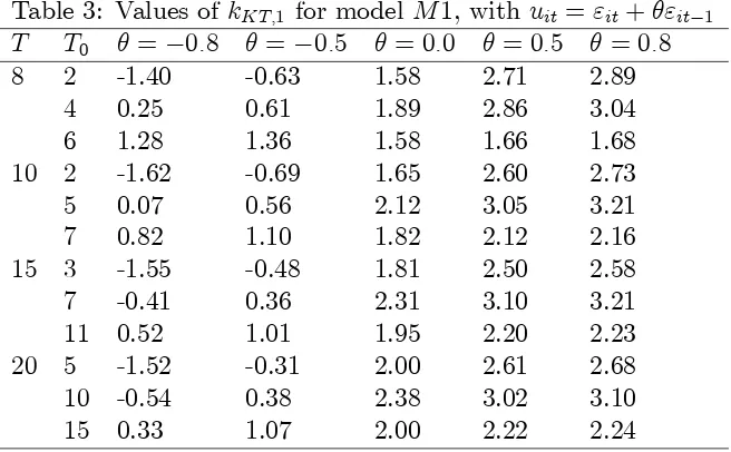
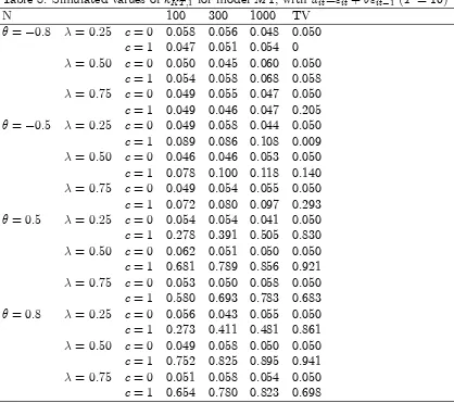
on the sign of _ts. To see this more clearly, in Table 3, we present estimates of the power

slope parameterkKT;1 assuming that error terms uit follow a MA(1) process:

uit="it+ "it 1,

where "it N IID(0; 2

"). Note that the table also considers the case that = 0 (i.e., there

is no serial correlation), but the KT test allows for serial correlation of order p = 1. This

case can show if the KT test loses signi…cant power if a higher order of serial correlation p

is assumed than the correct one. The results of the table also show that the KT test has

always power if 0 or the break point T0 is at the middle of the sample (i.e., = 0:5),

as in the case of no serial correlation (see Table 1). The …nding that the test has power

for unit roots even if higher than the correct order of serial correlation is assumed.6 _{As was}

expected, the power of the test in this case is always less compared to that when the correct

lag order p = 0 is considered. This can be attributed to the fact that the test exploits less

moment conditions in drawing inference about unit roots, by assuming p= 1 when = 0.

Another interesting conclusion that can be drawn from the results of the table is that,

when > 0, the power of the KT test becomes bigger than that of its version which does

not allow for serial correlation uit, presented in the previous section (see Table 2). We have

found that this result can be mainly attributed to the presence of terms tr( ( )_p;1 ) and

tr( 0 ( )

p;1 ) in the function of slope coe¢cient kKT;1, given by Theorem 3. These have a

positive e¤ect onkKT;1 (i.e., tr( ( )p;1 ) +tr( 0 ( )

p;1 )<0)when >0and a negative e¤ect

when <0 (i.e., tr( ( )_p;1 ) +tr( 0 ( )

p;1 )> 0).7 As T increases, the above sign e¤ects of

the sign of on the KT test are ampli…ed. These power gains of the KT test for model

M1, when > 0, may be also attributed to the fact that a positive value of adds to the

variability of individual panel seriesyit, driving further away the limiting distributions of the

test under the null and alternative hypotheses.

For model M2, the limiting distributions of the KT test under'_N = 1 pc

N and serially

correlated error terms uit are given in the next theorem. Note that, for this model, the

maximum order of serial correlation allowed by theKT test is given as

pmax = 8 > > <

> > :

T

2 3;if T is even andT0 =

T

2

min_fT0 2; T T0 2g otherwise;

6_{We have found that this is true even forp >1.} 7_{The sum of tracestr(F}0_Q( )

1 ) +tr( 0Q ( )

1 )a¤ects the power of theKT test, too. However, because this constitutes a parabola function which opens upwards, its e¤ect on kKT ;1 is almost symmetrical with respect to the sign of . Thus, the relationship betweenkKT ;1 and is mainly determined bytr( ( )p;1 ) +

tr( 0 ( )

see Karavias and Tzavalis (2012).

Theorem 4 Let conditions (b1)-(b6) of Assumption 1 hold. Then, under 'N = 1 pc_N, we

have

V_KT;( ) 1₂ =2^( )₂ pN '^( )₂ 1 ^b

( ) 2

^( )

2 !

d

!N( ckKT;2;1), for model M2,

as N _{! 1}, where

kKT;2 =

tr(F0_Q( )

2 ) +tr( 0Q ( )

2 ) tr(

( )

p;2 ) tr( 0 ( )

p;2 ) q

2tr((A( )_KT;2 )2₎

.

The results of the theorem indicate that, if it allows for serial correlation inuit, the KT

test can have non-trivial power even in the case of incidental trends. Table 4 presents values

of kKT;2 for the case that uit follows M A(1) process: uit = "it + "it 1. This is done for

di¤erent values of and T. As in Table 3, we also consider the case that = 0.

The results of Table 4 indicate that, for model M2, the KT test has non-trivial power

only if <0. If = 0, the test has trivial power while for >0, the test is biased. For <0,

the power of the test increases with T. For a given T; it becomes bigger if the break point

T0 is located towards the end of the sample, i.e. = 0:75. These results are in contrast to

those for model M1, presented in Table 3, where the KT test is found to have more power

if >0. This can be attributed to the interaction between matrix and annihilator matrix

Q( )₂ , entering the trace terms tr(:), on the power slope parameter kKT;2 and, in particular,

on terms tr( ( )_p;2 )and tr( 0_p;( )₂ ). Evaluations of these terms show that negative values

of reverse the power reduction e¤ects coming from detrending of the individual panel series

through matrix Q( )₂ . In contrast to model M1, this now happens only when <0. As for

the reduction in the variability of series yit, which a negative value of implies. The series

behave more like being generated from a model with a common trend. As shown by Moon

et al. (2007), in this case the incidental parameter problem disappears.

5

Monte Carlo results

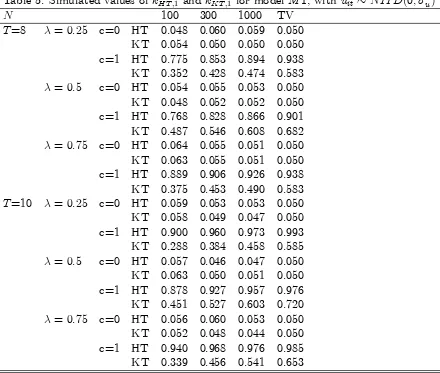
In this section, we conduct a Monte Carlo study to examine if the asymptotic local power

functions of the HT and KT tests, implied by the results of the previous section, provide

good approximations of their small sample ones. This is done based on 5000 iterations.

For each iteration, we calculate the size of the tests at 5% level (i.e., for c = 0) and their

power (i.e., for c = 1). This is done separately for the cases that uit N IID(0;1) and

uit = "it+ "it 1, with 2 f 0:8; 0:5;0;0:5;0:8g. The N and T-dimensions of the panel

data models are assumed as follows: N _{2 f}100;300;1000_gand T _{2 f}8;10;15;20_g, while the

break fraction is taken to be _{2 f}[0:25T];[0:5T];[0:75T]_g, where [ ] denotes integer part.

The nuisance parameters of the models are set to the following values: yi0 = 0,a( )i = 0 and

( )

i = 0; for all i, as they do not a¤ect the limiting distribution of the tests.

Tables 5 and 6 present the results of our simulation study for the case that uit

N IID(0;1). The last column of the tables gives the theoretical values (T V) of the power

function and the nominal size of the tests, at a= 5%. For model M1, the results of Table 6

indicate that both the HT and KT tests have size and power values which are very close to

their theoretical ones. Furthermore, the results con…rm that the HT test has more power

towards the beginning and the end of the sample while the KT test has more power in the

middle. As was also predicted by the theory, the HT test has higher power than the KT

local power function (see column T V) even for small N (e.g., N=100). However, this is

not always true for the KT test, which needs very high N in order its power to converge

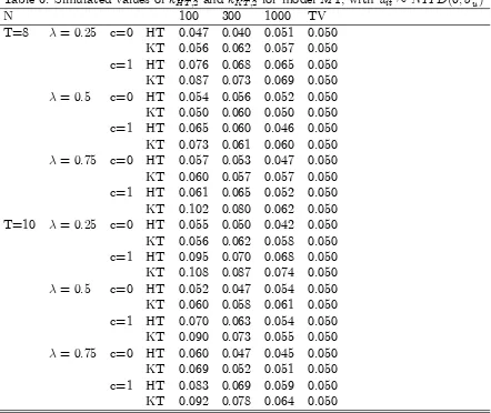
to its theoretical value. For model M2, the results of Table 6 indicate that, for large N,

both HT and KT tests have trivial power, as it was expected. However, in small samples

(e.g., N = 100), both tests have some non-trivial power. This can be obviously attributed

to second, or higher, order e¤ects of the true power function, which cannot be approximated

by the …rst-order approximation considered in our analysis. Note that, for model M2, the

KT test has slightly higher small sample power than theHT.

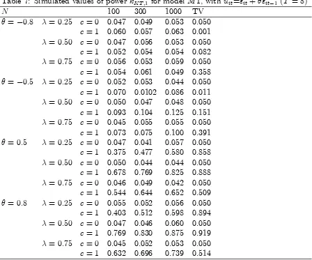
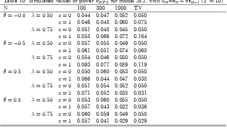
Tables 7, 8, 9 and 10 present the results of our simulation study for theKT test allowing

for serial correlation in error terms uit, assuminguit ="it+ "it 1. This is done for models

M1 and M2, and T _{2 f}8;10_g. The maximum order of serial correlation allowed by the

KT test is set to p = 1, which matches that of the MA process of uit. The results of these

tables are also consistent with theory. For model M1, the KT test has signi…cant power

when >0. This converges to its theoretical value, reported in the last column of the table,

quite fast as N increases. For negative values of , the test has also signi…cant power. This

happens for =_f0:75_g, as was predicted by the theory. Note that both the theoretical and

small sample values of the power function of the KT are higher than their corresponding

values in the absence of serial correlation (see Table 5). This is also consistent with the

theory and can be attributed to the serial correlation e¤ects of uit on the power function of

the test, discussed in the previous section.

For modelM2, the results of Tables 9 and 10 indicate that theKT test has smaller power

than for model M1. As was expected by the theory, the power of the test is non-trivial if

< 0. The KT test has also some small sample power if > 0, which quali…es its use in

e¤ects of the true power function, which are not approximated e¢ciently by our asymptotic

approximations. Finally, another interesting conclusion which can be drawn from the results

of our simulation study reported in Tables (7)-(10) is that, when <0, a break towards the

end of the sample increases the power of theKT test. When >0, the power of the test is

maximized at the middle of the sample. These results apply to both models M1 and M2.

They are also consistent with the theoretical results reported in Table 4.

6

Conclusions

This paper analyzes the asymptotic local power properties of least-squares based …xed-T

panel unit root tests allowing for a structural break in the deterministic components of the

AR(1) panel data model, namely its individual e¤ects and/or slope coe¢cients of its

indi-vidual linear (incidental) trends. This is done by assuming that the cross-section dimension

of the panel data models (N) grows large. Thus, the results of our analysis concern mainly

applications of the above tests to short panels, often used in empirical microeconomic studies.

The paper derives the limiting distributions under the sequence of local alternatives of

extensions of Harris and Tzavalis (1999) panel unit root tests (denoted as HT) allowing for

a structural break (see Karavias and Tzavalis (2013)) and Karavias’ and Tzavalis (2012)

recently developed panel data unit root tests (denoted as KT). In addition to a structural

break, the last test also allows for serial correlation in the error terms of the AR(1) panel

data model. Both of these tests are based on the least squares dummy variables estimator

of the autoregressive coe¢cient of the AR(1) panel data model which is corrected for its

inconsistency due to the deterministic components of the panel and/or serial correlation

The results of the paper lead to a number of interesting conclusions. First, they show

that, for the standard AR(1) panel data model with white noise error terms and individual

e¤ects, both the HT and KT tests have signi…cant asymptotic local power. The HT test

has much higher power than theKT. The power of this test increases withT, in contrast to

theKT test. The latter is found to be more appropriate for smallT. This happens because,

to adjust for the inconsistency of the least squares estimator, theKT test requires consistent

estimation of the variance of the error term, which leads to a reduction of its power. TheHT

test does not depend on this nuisance parameter, as it adjusts the least squares estimator

for both the inconsistency of its numerator and denominator, and thus the variance of the

error term is cancelled out. The HT test is found to have more power when the break is

towards the beginning or the end of the sample, while the KT test has more power when

the break is towards the middle of the sample.

Second, both the HT and KT tests have asymptotically trivial power in the case that

the AR(1) allows also for incidental trends. The allowance for a common break in the slope

coe¢cients of the incidental trends does not change the behavior of the tests. This problem

does not always exist for theKT test extended for serial correlation of the error term. In this

case, the paper presents circumstances that theKT test has non-trivial power. In particular,

this happens when the error term follows a MA(1) procedure with negative serial correlation.

The power of theKT in this case can be attributed to the e¤ects of the serial correlation of

error term on the adjustment of the least squares estimator of the autoregressive coe¢cient

for its inconsistency, upon which the KT test is based on. In contrast to large-T panel

data unit root tests, the power function of …xed-T tests depend on the values of nuisance

parameters capturing serial correlation e¤ects which can a¤ect the asymptotic (overN) power

This exercise has shown that the empirical probabilities of rejection are very close to their

theoretical values, which means that the asymptotic theory provides a good approximation

of small sample results of …xed-T panel data unit roots.

References

[1] Arellano, M., 2003, Panel data econometrics, Oxford University Press, UK

[2] Bai J., Carrion-I-Silvestre, J.L., 2009. Structural Changes, Common Stochastic Trends,

and Unit Roots in Panel Data. Review of Economic Studies, vol. 76(2), 471-501.

[3] Carrion-i-Silvestre, J.L., Del Barrio-Castro, T., Lopez-Bazo, E., 2005. Breaking the

panels: An application to real per capita GDP. Econometrics Journal, 8, 159-175.

[4] Chan, F., Pauwels, L.L., 2011. Model speci…cation in panel data unit root tests with an

unknown break. Mathematics and Computers in Simulation. 81, 1299–1309.

[5] Hahn, J., Kuersteiner, G., 2002. Asymptotically unbiased inference for a dynamic panel

model with …xed e¤ects when both n and T are large. Econometrica. 70, 1639-1657.

[6] Hadri K., Larsson, R., Rao, Y., 2012. Testing for stationarity with a break in panels

where the time dimension is …nite. Bulletin of Economic Research, 64, s123-s148.

[7] Harris D., Harvey D., Leybourne S., and Sakkas N., 2010. Local asymptotic power of the

Im-Pesaran-Shin panel unit root test and the impact of initial observations. Econometric

[8] Harris, D., Leybourne, S., and McCabe, B., 2005. Panel Stationarity Tests for

Purchas-ing Power Parity with Cross-Sectional Dependence. Journal of Business & Economic

Statistics, vol. 23, 395-409.

[9] Harris, R., Tzavalis, E., 1999. Inference for unit roots in dynamic panels where the time

dimension is …xed. Journal of Econometrics, 91, 201-226.

[10] Harris, R., Tzavalis, E., 2004. Inference for unit roots for dynamic panels in the

pres-ence of deterministic trends: Do stock prices and dividends follow a random walk ?

Econometric Reviews 23, 149-166.

[11] Harvey, D.I., Leybourne S.J., 2005. On testing for unit roots and the initial observation.

Econometrics Journal 8, 97–111.

[12] Karavias, Y., and Tzavalis, E., 2012. Generalized …xed-T Panel Unit Root Tests

Allow-ing for Structural Breaks. Granger Centre Discussion Paper Series, No 12/02.

[13] Karavias, Y., and Tzavalis, E., 2013. Testing for unit roots in short panels

allow-ing for structural breaks. Computational Statistics and Data Analysis. (In press).

http://dx.doi.org/10.1016/j.csda.2012.10.014

[14] Kruiniger, H., 2008. Maximum Likelihood Estimation and Inference Methods for the

Covariance Stationary Panel AR(1)/Unit Root Model. Journal of Econometrics 144,

447-464.

[15] Kruiniger, H., and E., Tzavalis, 2002. Testing for unit roots in short dynamic panels

with serially correlated and heteroscedastic disturbance terms. Working Papers 459,

[16] Madsen E., 2010. Unit root inference in panel data models where the time-series

dimen-sion is …xed: a comparison of di¤erent tests. Econometrics Journal 13, 63-94.

[17] Meligkotsidou, L., Tzavalis, E., Vrontos I.D., 2011. A Bayesian analysis of unit roots

and structural breaks in the level, the trend and the error variance of autoregressive

models of economic series. Econometric Reviews, 30 (2), 208-249.

[18] Moon, H.R., Perron, B., 2008. Asymptotic local power of pooled t-ratio tests for unit

roots in panels with …xed e¤ects. Econometrics Journal 11, 80-104.

[19] Moon, H.R., Perron, B., Phillips, P.C.B., 2007. Incidental trends and the power of panel

unit root tests. Journal of Econometrics, 141(2), 416-459.

[20] Pauwels, L.L., Chan, F., Mancini, G.T., 2012. Testing for Structural Change in

Hetero-geneous Panels with an Application to the Euro’s Trade E¤ect. Journal of Time Series

Econometrics, 4(2), Article 3.

[21] Perron, P., 1989. The great crash, the oil price shock, and the unit root hypothesis.

Econometrica, 57, 1361-1401.

[22] Schott, J.R., 1996. Matrix Analysis for Statistics, Wiley-Interscience.

6.1

Appendix

In this appendix, we provide proofs of the theorems and the corollary presented in the main

text of the paper.

Proof of Theorem 1: First, we derive the limiting distribution of theHT test statistic,

under the sequence of local alternatives'_N = 1 _pc

N. De…ne vectorw= (1; 'N; '

2

and matrix

=

0

B B B B B B B B B B B B B B B B B B B B B B @

0 : : : : : 0

1 0 :

'_N 1 : :

'2

N 'N : : :

: : : : :

: : 1 0 :

'T_N 2 'T_N 3 : : 'N 1 0

1

C C C C C C C C C C C C C C C C C C C C C C A

Under null hypothesis H0: c = 0; we have = : The …rst order Taylor expansions of

and w yields

= +F('N 1) +op(1) and (5)

w = e+f('_N 1) +oP(1), (6)

respectively, whereF = _d'd

N jc=0 and f =

dw

d'N jc=0. Based on the above de…nitions ofw and

, vectoryi 1 can be written as

yi 1 =wyi0+ X1( ) ( )

i + ui, (7)

where ( )_i = (a(1)_i (1 '_N); a(2)_i (1 '_N))0 _{= (1 '}

N)(a

(1)

i ; a

(2)

yi 1, the HT test statistic for model M1 can be written under'N = 1 pc_N as follows:

p

N(^'( )₁ '_N B1( )) (8)

= pN

0 B B B B @ 1 N N X i=1 y0

i 1Q ( )

1 ('Nyi 1+X1( ) ( )

i +ui)

1 N N X i=1 y0

i 1Q ( ) 1 yi 1

'_N B1( ) 1 C C C C A ;

= pN

0 B B B B @ 1 N N X i=1 y0

i 1Q ( ) 1 ui 1 N N X i=1 y0

i 1Q ( ) 1 yi 1

B1( ) 1 N N X i=1 y0

i 1Q ( ) 1 yi 1

1 N N X i=1 y0

i 1Q ( ) 1 yi 1

1 C C C C A ; = 1 p N N X i=1 y0

i 1Q ( )

1 ui p1_NB1( )

N

X

i=1

y0

i 1Q ( ) 1 yi 1

1 N N X i=1 y0

i 1Q ( ) 1 yi 1

= (A) (B)

(C) : (9)

Next, we derive asymptotic results of each of quantities (A); (B) and (C), de…ned by (9).

Substituting (7) in(A), we have

(A) _p1

N N

X

i=1

y0

i 1Q ( ) 1 ui =

1 p N N X i=1

yi0w0+ ( )i 0X

( )0

1 0+u0i 0 Q

( ) 1 ui

= _p1

N N

X

i=1

yi0w0Q( )1 ui+ ( )i 0X

( )0

1 0Q ( )

1 ui+u0i 0Q

( ) 1 ui

Using relationships (5)-(6), we can …nd the following limits of the summands entering into

the last relationship of (A). First, it can be shown that

1 p N N X i=1

yi0w0Q( )1 ui =

1 p N N X i=1

yi0(e0+f0('N 1))Q

( )

1 ui+oP(1);

= p1

N N

X

i=1

yi0e0Q( )1 ui+

c N

N

X

i=1

yi0f0Q( )1 ui+oP(1);

since e0_Q( )

1 = 0 and E(yi0ui) = 0 by assumption (b5), and

1 p N N X i=1 ( )0

i X

( )0

1 0Q ( ) 1 ui

= _p1

N N

X

i=1 ( )0

i X

( )0

1 ( 0+F0('N 1) +op(1))Q

( ) 1 ui;

= _p1

N N

X

i=1 ( )0

i X

( )0

1 0Q ( ) 1 ui+

c N

N

X

i=1 ( )0

i X

( )0

1 F0Q ( )

1 ui+op(1);

= c

N N

X

i=1

(a(1)_i ; a(2)_i )0X₁( )0 0_Q( )

1 ui+

c2

N3=2

N

X

i=1

(a(1)_i ; a(2)_i )0X₁( )0F0_Q( )

1 ui+op(1);

= op(1); (11)

since E(a( )_i ui) = 0 by assumption (b5). Finally, we have

1 p N N X i=1 u0

i 0Q

( ) 1 ui =

1 p N N X i=1 u0

i( 0 +F0('N 1) +op(1))Q

( ) 1 ui;

= _p1

N N

X

i=1

u0

i 0Q

( ) 1 ui c N N X i=1 u0

iF0Q

( )

1 ui+op(1);

where c N N X i=1 u0

iF0Q

( ) 1 ui

p

!c 2utr(F0Q

( )

1 ) and (12)

p N 1 N N X i=1 u0

i 0Q

( )

1 ui 2utr( 0Q

( ) 1 )

!

d

!N(0; VHT;A); (13)

whereVHT;Ais the variance of the last limiting distribution. Based on the asymptotic results

given by equations (10)-(13), we can show that

(A) _p1

N N

X

i=1

y0

i 1Q ( ) 1 ui

d

!N c 2_utr(F0_Q( )

To derive asymptotic results for summand (B), write it as follows:

(B) _p1

NB1( ) N

X

i=1

y0

i 1Q ( ) 1 yi 1

= p1

NB1( ) N

X

i=1

yi0w0+ ( )i 0X

( )0

1 0+u0i 0 Q

( )

1 yi0w+ X1( ) ( )

i + ui :

By similar arguments to those applied to derive results (10)-(13), we can prove the following

asymptotic results: 1 p N N X i=1

y_i2₀w0_Q( )

1 w+yi0w0Q( )1 X ( ) 1

( )

i +yi0w0Q( )1 ui = op(1);(15)

1 p N N X i=1 ( )0

i X

( )0

1 0Q ( ) 1 wyi0+

( )0

i X

( )0

1 0Q ( )

1 X

( ) 1

( )

i + X

( ) 1

( )

i ui) = op(1);(16)

1 p N N X i=1 u0

i 0Q

( )

1 wyi0+u0i 0Q

( )

1 X

( ) 1

( )

i = op(1);(17)

1 p N N X i=1 u0

i 0Q

( ) 1 ui =

1 p N N X i=1 u0

i( 0+F0('N 1))Q

( )

1 ( +F('N 1))ui +op(1); (18)

where p N 1 N N X i=1 u0

i 0Q

( )

1 ui 2utr( 0Q

( )

1 )

!

d

!N(0; VHT;B); (19)

c N N X i=1 u0

iF0Q

( ) 1 ui

p

! 2utr(F0Q

( )

1 ); (20)

c N N X i=1 u0

i 0Q

( ) 1 F ui

p

! 2utr( 0Q

( )

1 F) and (21)

c2

N3=2

N

X

i=1

u0

iF0Q

( )

Based on the above results, given by equations (15)-(22), it can be shown that

(B) _p1

NB1( ) N

X

i=1

y0

i 1Q ( ) 1 yi 1

d

! (23)

N c 2_uB1( )[tr(F0Q( )1 ) +tr( 0Q ( )

1 F)]; B12( )VHT;B :

Finally, following similar arguments to the above, we can easily show that, for quantity (C),

the following asymptotic result holds:

(C) 1

N N

X

i=1

y0

i 1Q ( ) 1 yi 1

p

! 2utr( 0Q

( )

1 ): (24)

Using asymptotic results (14), (23) and (24), equation (9) implies that

p

N(^'( )₁ '_N B₁( ))_!d N ctr(F

0_Q( )

1 ) 2B1( )tr(F0Q( )1 )

tr( 0_Q( )

1 )

; V_HT;( )₁

!

; (25)

orpN(^'( )₁ 1 B1( ))!d N c

tr(F0_Q( )

1 ) +tr( 0Q ( )

1 ) 2B1( )tr(F0Q( )1 )

tr( 0_Q( )

1 )

; V_HT;( )₁

!

;

sincetr( 0_Q( )

1 ) B1( )tr( 0Q( )1 ) = 0. Note that the analytic formula of varianceV ( )

HT;1 of

the last limiting distribution is the same with that of the HT test under null hypothesisH0:

c= 0, given byV_HT;( )₁ = 2tr(A

( )2

HT ;1)

tr( 0_Q( )

1 )2

. This does not depend on local parameterc. It remains

the same under the null and sequence of local alternative hypotheses (see, e.g., Madsen

(2010) and Karavias and Tzavalis (2013)), given as V_HT;( )₁ = 2tr(A

( )2

HT ;1)

tr( 0_Q( )

1 )2

the above limiting distribution yields

V_HT;( ) 1₁ =2pN(^'( )₁ 1 B1( ))

d

!N( ckHT;1;1), with (26)

kHT;1 =

tr(F0_Q( )

1 ) +tr( 0Q ( )

1 ) 2B1( )tr(F0Q( )1 ) q

2tr(A( )_HT;2₁)

.

Substituting into the above formula ofkHT;1 the following identities:

tr(F0_Q( )

1 ) = tr( 0Q ( )

1 F) = (27)

= 6 144(3

2

3 + 1)T3 1

12(2

2

2 + 1)T2 1

24T + 1 6

tr( 0_Q( )

1 ) +tr(F0Q ( )

1 ) +tr( 0Q ( )

1 ) = 0; (28)

tr(F0_Q( )

1 ) =

T2

6 (2

2 _{2 + 1) +} T

2 4

6; (29)

tr( 0_Q( )

1 ) =

T 2

2 ; (30)

tr( 0_Q( )

1 ) =

T2

6 (2

2 _{2 + 1)} 2

6; (31)

tr(A( )_HT;2₁) = tr

"

1 2(

0_Q( )

1 +Q ( )

1 ) B1( )( 0Q( )1 ) 2#

;

(32)

tr 0_Q( )

1 +Q ( ) 1 2 = T 2 6 (2 2

2 + 1) +T 7

3; (33)

tr 0_Q( )

1 2

= 1 90(2

4 ₄ 3_{+ 6} 2 _{4 + 1)T}4 ₍₃₄₎

+ 1 36(2

2 _{2 + 1)T}2 7

90;

tr 0_Q( )

1 +Q ( )

1 0Q

( )

1 =

T 2

2 ; (35)

analytically written as

2tr(A( )_HT;2₁) = D

S, where

D = T6R1 +T5R2+T4R3+T2R4+ 216T 136;

S = T4 1+T2 2+ 240;

R1 = 40 6 120 5+ 204 4 208 3+ 162 2 78 + 17;

R2 = 216 4+ 432 3 528 2+ 312 78;

R3 = 216 4 432 3 + 588 2 372 + 108;

R4 = 120 2+ 120 144;

1 = 240 4 480 3 + 480 2 240 + 60and

2 = 480 2+ 480 240.

To derive the limiting distribution of theKT test under the sequence of local alternatives

'_N = 1 _pc

N, write

^( )

1

p

N '^( )₁ ^b

( ) 1 ^( ) 1 '_N !

= ^( )₁ pN

0 B B B B @

'_N +

1 N N X i=1 y0

i 1Q ( ) 1 ui 1 N N X i=1 y0

i 1Q ( ) 1 yi0 1

^_b( ) 1 ^( ) 1 '_N 1 C C C C A ;

= pN 1 N

N

X

i=1

y0

i 1Q ( )

1 ui ^2utr( 0Q

( ) 1 )

!

;

= pN 1 N

N

X

i=1

y0

i 1Q ( ) 1 ui 1 N N X i=1 y0 i ( ) 1 yi ! ;

= p1

N N

X

i=1

y0

i 1Q ( ) 1 ui 1 p N N X i=1 y0 i ( )

where yi can be written as

yi =ui+ ('_N 1)yi 1+X1( ) ( )

i : (37)

The limiting distribution of the KT test under '_N = 1 _pc

N can be proved by obtaining

asymptotic results for the two summands entering into equation (36), i.e., p1

N N

X

i=1

y0

i 1Q ( ) 1 ui

and p1

N N

X

i=1

y0

i

( )

1 yi, following analogous to the proof of (26) steps. The formula of slope

power parameter kKT;1 is given as

kKT;1 =

tr(F0_Q( )

1 ) +tr( 0Q ( )

1 )

q

2tr(A( )_KT;2₁)

: (38)

Substituting the following identities into the above formula of kKT;1:

tr(A( )_KT;2₁) = tr 1

2(

0_Q( )

1 +Q ( ) 1

( ) 1

( )0

1 ) 2!

; (39)

tr( ( )₁ ) = tr( 0 ( )

1 ) = 0; (40)

2tr(A( )_KT;2₁) = 2tr(P( )) 2tr(Z( )2); with Z( ) = 1 2(

( )0

1 +

( )

1 ) (41)

and P( ) = 1 2(

0_Q( )

1 )2+

1 2

0_Q( )

1 ; (42)

tr ( 0_Q( )

1 )2 =

T2

12(2

2 _{2 1) +} T

2 5

6 and (43)

tr(Z( )2) =

1

T + 2( 1) T

6( 1) 1 (44)

yields the results of Theorem 1, for the KT statistic.

(1) can be derived based on analogous arguments to those applied for the proof of Theorem

1.

To obtain the analytic formula ofk_HT;1, given by equation (1), scale (8) byT, replace'N

with '_N;T, and apply asymptotic theory forN _{! 1}, as in Theorem 1. Then, we will have

TpN(^'( )₁ '_N;T B1( ))

d

!N ctr(F

0_Q( )

1 ) 2B1( )tr(F0Q( )1 )

tr( 0_Q( )

1 )

; T2V_HT;( )₁

!

:

Multiplying with T2_V( )

HT;1 1=2

and using = 1 _Tpc

N, the last limiting distribution can be

written as

T T2V_HT;( )₁ 1=2pN(^'( )₁ 1 B1( ))

d

!N c1

TkHT;1;1 (45)

where kHT;1 = tr(F

0_Q( )

1 )+tr( 0Q ( )

1 ) 2B1( )tr(F0Q( )1 )

r

2tr(A( )2_{HT ;1})

(see proof of Theorem 1). By taking the

limit for T _{! 1} of kHT;1 and T2VHT;( )1; (45) can be written as

T V_HT;( )₁ 1=2pN(^'( )₁ 1 B1( ))

d

!N ck_HT;1;1 , where

k_HT;1 lim

T

1

TkHT;1 =

3 2 3 + 1 4(2 2 2 + 1)

r 1

R1

and

V_HT;( )₁ lim

T T

2_V( )

HT;1 =

36R1

1(2 2 2 1)2

:

The analytic formulas of the last two limits are derived based on the results of identities

(27)-(35). The above results have been derived by taking limits sequentially, …rst forN _{! 1}and

then for T _{! 1}. Joint convergence in N; T requires the extra assumption that p_TN _! 0,

see also Moon and Perron (2008). However, forc= 0 there is no need to specify the relative

Tzavalis (2013)).

The formulas of k_KT;1 and V_KT;( )₁, given by the corollary for the large-T version of the

KT test, can be derived by following similar steps to the above. Then, using the results of

identities (39)-(44), we can obtain

k_KT;1 lim

T

1

TkKT;1 = 0 and V

( )

KT;1 lim

T T

2_V( )

KT;1

36(2 4 4 3+ 3 2 ) 12( 1) (2 2 2 + 1)2:

Proof of Theorem 2: To prove the theorem, we will follow analogous steps to those for

the proof of Theorem 1. We now will rely on relationships (7) and (37), where now vector

( )

i is de…ned as

( )

i =

0

B B B B B B B B B B @

(1 '_N)a(1)_i +'_N (1)_i

(1 'N)a

(2)

i +'N

(2)

i

(1 '_N) (1)_i

(1 '_N) (2)_i

1

C C C C C C C C C C A

=e i+ (1 'N) i,

due to the presence of individual trends under'N;T = 1 _Tpc_N, where i = (

(1)

i

(1)

i ;

(2)

i

(2)

i ;

(1)

i ;

(2)

i )0; e =

0

B B @

1 0 0 0

0 1 0 0

1

C C

A and i = ( (1)i ;

(2)

statistic for model M2 can be written as follows:

p

N(^'( )₂ '_N B2( ))

= pN

0 B B B B @ 1 N N X i=1 y0

i 1Q ( )

2 ('Nyi 1+X2( ) ( )

i +ui)

1 N N X i=1 y0

i 1Q ( ) 2 yi 1

'_N B2( ) 1 C C C C A = 1 p N N X i=1 y0

i 1Q ( )

2 ui p1_NB2( )

N

X

i=1

y0

i 1Q ( ) 2 yi 1

1 N N X i=1 y0

i 1Q ( ) 2 yi 1

= (A

0

) (B0)

(C0

) ,

where(A0) p1

N N

X

i=1

y0

i 1Q ( ) 2 ui,(B

0

) p1

NB2( ) N

X

i=1

y0

i 1Q ( )

2 yi 1and(C

0

) _N1

N

X

i=1

y0

i 1Q ( ) 2 yi 1.

As in the proof of Theorem 1, next we derive asymptotic results of(A0),(B0)and (C0), using

( )

i =e i+ (1 'N) i. The most important ones are the following:

p N 1 N N X i=1 0

ie0X

( )0

2 0Q ( )

2 X

( )

2 e i tr(e0X2( )0 0Q ( )

2 X

( )

2 e E( i 0i))

!

d

!N(0; VHT;4)

c N N X i=1 0

ie0X

( )0

2 F0Q ( )

2 e i

p

!ctr(e0_X( )0

2 F0Q ( )

2 e E( i 0i))

c N N X i=1 0

ie0X

( )0

2 0Q ( ) 2 F X

( ) 2 e i

p

!ctr(e0_X( )0

2 0Q ( )

2 F e E( i 0i))

c N N X i=1 0 iX

( )0

2 0Q ( )

2 X

( ) 2 e i

p

!ctr(X2( )0 0Q ( )

2 X

( )

2 e E( i 0i))

c N N X i=1 0

ie0X

( )0

2 0Q ( )

2 X

( ) 2 i

p

!ctr(e0_X( )0

2 0Q ( )

2 X

( )

2 E( i 0i))

after using the following identities:

tr(e0_X( )0

2 0Q ( )

2 X

( )

2 e E( i 0i)) = 0

tr(e0_X( )0

2 F0Q ( )

2 e E( i 0i)) tr(e0X

( )0

2 0Q ( )

2 F e E( i 0i)) = 0

and tr(X₂( )0 0_Q( )

2 X

( )

2 e E( i 0i)) tr(e0X

( )0

2 0Q ( )

2 X

( )

2 E( i 0i)) = 0.

The proof of the second result of the theorem, i.e., kKT;2 = 0, can be proved by following

analogous steps to the above and using the following identities:

tr(e0_X( )0

2 ( )

2 X

( )

2 e E( i 0i)) tr(e0X

( )0

2 0

( ) 2 X

( )

2 e E( i 0i)) = 0

and tr(X₂( )0 ( )₂ X₂( )e E( i 0i)) tr(e0X

( )0

2 ( ) 2 X

( )

2 E( i 0i)) = 0.

Proof of Theorem 3: This can be proved by following analogous steps to the proof of

Theorem 1, for the KT test statistic, by setting E(uiu0

i) = instead of 2uIT:

Proof of Theorem 4: This can be proved by following analogous steps to the proof of

7

Tables

Table 1: Values ofkHT;1 and kKT;1 for model M1

kHT;1 kKT;1

nT 8 10 15 20 8 10 15 20 0.25 3.18 4.12 6.11 7.75 1.85 1.86 1.96 2.10 0.50 2.93 3.62 5.32 6.99 2.12 2.23 2.34 2.39 0.75 3.18 3.81 5.78 7.75 1.85 2.04 2.09 2.10

Table 2: Values of slope parameters k_HT;1 and k_KT;1

0.10 0.20 0.30 0.40 0.50 0.60 0.70 0.80 0.90

k_HT 0.433 0.394 0.360 0.338 0.332 0.338 0.360 0.394 0.433

k_KT 0 0 0 0 0 0 0 0 0

Table 3: Values ofkKT;1 for model M1, withuit ="it+ "it 1

T T0 = 0:8 = 0:5 = 0:0 = 0:5 = 0:8

8 2 -1.40 -0.63 1.58 2.71 2.89

4 0.25 0.61 1.89 2.86 3.04

6 1.28 1.36 1.58 1.66 1.68

10 2 -1.62 -0.69 1.65 2.60 2.73

5 0.07 0.56 2.12 3.05 3.21

7 0.82 1.10 1.82 2.12 2.16

15 3 -1.55 -0.48 1.81 2.50 2.58

7 -0.41 0.36 2.31 3.10 3.21

11 0.52 1.01 1.95 2.20 2.23

20 5 -1.52 -0.31 2.00 2.61 2.68

10 -0.54 0.38 2.38 3.02 3.10

15 0.33 1.07 2.00 2.22 2.24

Table 4: Values ofkKT;2 for model M2, withuit ="it+ "it 1

T T0 = 0:8 = 0:5 = 0:0 = 0:5 = 0:8

8 4 0:08 0:070 0 0:09 0:11 10 5 0:20 0:15 0 0:12 0:14 7 0:66 0:46 0 0:21 0:24

15 3 0 0 0 0 0

Table 5: Simulated values ofkHT;1 and kKT;1 for model M1, with uit N IID(0; 2u)

N 100 300 1000 TV

T=8 = 0:25 c=0 HT 0.048 0.060 0.059 0.050 KT 0.054 0.050 0.050 0.050 c=1 HT 0.775 0.853 0.894 0.938 KT 0.352 0.428 0.474 0.583

= 0:5 c=0 HT 0.054 0.055 0.053 0.050 KT 0.048 0.052 0.052 0.050 c=1 HT 0.768 0.828 0.866 0.901 KT 0.487 0.546 0.608 0.682

= 0:75 c=0 HT 0.064 0.055 0.051 0.050 KT 0.063 0.055 0.051 0.050 c=1 HT 0.889 0.906 0.926 0.938 KT 0.375 0.453 0.490 0.583

T=10 = 0:25 c=0 HT 0.059 0.053 0.053 0.050 KT 0.058 0.049 0.047 0.050 c=1 HT 0.900 0.960 0.973 0.993 KT 0.288 0.384 0.458 0.585

= 0:5 c=0 HT 0.057 0.046 0.047 0.050 KT 0.063 0.050 0.051 0.050 c=1 HT 0.878 0.927 0.957 0.976 KT 0.451 0.527 0.603 0.720

Table 6: Simulated values ofkHT;2 and kKT;2 for model M1, with uit N IID(0; 2u)

N 100 300 1000 TV T=8 = 0:25 c=0 HT 0.047 0.040 0.051 0.050

KT 0.056 0.062 0.057 0.050 c=1 HT 0.076 0.068 0.065 0.050 KT 0.087 0.073 0.069 0.050

= 0:5 c=0 HT 0.054 0.056 0.052 0.050 KT 0.050 0.060 0.050 0.050 c=1 HT 0.065 0.060 0.046 0.050 KT 0.073 0.061 0.060 0.050

= 0:75 c=0 HT 0.057 0.053 0.047 0.050 KT 0.060 0.057 0.057 0.050 c=1 HT 0.061 0.065 0.052 0.050 KT 0.102 0.080 0.062 0.050 T=10 = 0:25 c=0 HT 0.055 0.050 0.042 0.050 KT 0.056 0.062 0.058 0.050 c=1 HT 0.095 0.070 0.068 0.050 KT 0.108 0.087 0.074 0.050

= 0:5 c=0 HT 0.052 0.047 0.054 0.050 KT 0.060 0.058 0.061 0.050 c=1 HT 0.070 0.063 0.054 0.050 KT 0.090 0.073 0.055 0.050