Image Motion Deblurring Based on Salient Structure Selection and L0 2 Norm Kernel Estimation

http://www.scirp.org/journal/jcc ISSN Online: 2327-5227

ISSN Print: 2327-5219

Image Motion Deblurring Based on

Salient Structure Selection and

L

0−2

Norm Kernel Estimation

Fuwei Zhang, Yumin Tian

Xidian University, Xi’an, China

Abstract

Single image motion deblurring has been a very challenging problem in the field of image processing. Although there are many researches had been pro-posed to solve this problem, it still has problems on kernel accuracy. In order to improve the kernel accuracy, an effective structure selection method was used to select the salient structure of the blur image. Then a novel kernel es-timation method based on L0 2− norm was proposed. To guarantee the

sparse kernel and eliminate the negative influence of details L0-norm was

used. And L2-norm was used to ensure the continuity of kernel. Many

expe-riments were done to compare proposed method and state-of-the-art me-thods. The results show that our method can estimate a better kernel and use less time than previous work, especially when the size of blur kernel is large.

Keywords

Motion Deblurring, Structure Selection, Kernel Estimation

1. Introduction

Motion blur is caused by the relative displacement between the camera and the target due to the camera or a hand shake. With the popularity of the camera in recent years, the blur is very common in life, so it’s important for the image mo-tion deblurring. However, momo-tion deblurring is a completely challenging prob-lem since it’s an ill-posed probprob-lem. Ordinarily, if the motion blur is shift-inva- riant, the image blur process can be modeled as:

g= ⊗ +f k n

where g is the known blur image, f is the latent image, k is a motion blur kernelor a point spread function(PSF), n is noise produced during image

ac-How to cite this paper: Zhang, F.W. and Tian, Y.M. (2017) Image Motion Deblur-ring Based on Salient Structure Selection and L0−2 Norm Kernel Estimation. Journal of Computer and Communications, 5, 24- 32.

https://doi.org/10.4236/jcc.2017.53003

quisition, ⊗ is the convolution operator. In general, the image deblurring could be divided into two types-non-blind: deconvolution and blind deconvolu-tion. In non-blind image deblurring method, the blur kernel and blurred image are known, and the major problem is the deconvolution. In the blind image me-thod, the kernel is usually unknown when the blurred image is acquired in life. In this paper, we are more concerned about the blind image. One of the most difficult problem of the blind image deblurring method is the available informa-tion is too little, only one blurred image, we need to estimate the blur kernel from the blurred image, and then restore the latent image by the deconvolution operation of the kernel and the blurred image.

The kernel estimation is an important step in the deblurring process, since the kernel will impact directly on the restoration of latent image. The awful or inac-curate kernel will produce ringing artifact in the latent image. At the beginning, the researchers used some regularization to estimate the accurate kernel [5] [9], but this approach is very costly. Cho [2] used bilateral filtering and shock filter-ing to predict the image edges for the kernel estimation, but this method is too simple.

Now, we use a more effective image structure extraction algorithm. It avoids the negative effect of the details on the kernel estimation. Meanwhile, we pro-pose a novel method of kernel estimation, it can not only estimate the kernel much faster but also suppress the noise, and guarantee the continuity of kernel. The coarse-to-fine iterative process is taken. The image structure is selected from the blurred image. Then, the kernel can be obtained from the image struc-ture. The latent image, which be got from the estimated kernel and the given blurred image, is prepared for the next finer level.

2. Related Work

deblurring speed, and had a wonderful result. Xu & Jia [9] discovered that these details had a negative impact on the kernel estimation, so they used a model based on image gradient to eliminate the details, and ISD was employed to refine the kernel. Pan et al. [7] proposed an algorithm which utilized the salient struc-ture to estimate the kernel, it could get better results when the kernel size is large and the blurred image had complex structure, but it need a lot of time when the kernel size is large. Long et al. [6] proposed a kernel fusion method which used several state-of-the-art motion deblurring methods to estimate the kernel. They trained a more precise kernel via the several kernel results. However this ap-proach was dependent on these state-of-the-art methods.

3. Our Method

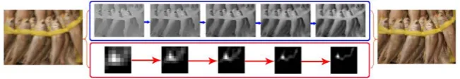
Our method focuses on the salient structure selection and the kernel estimation. An effective salient structure extraction method is critical to the kernel estima-tion, and the accurate kernel is indispensable to the deconvolution. Figure 1 shows the image structure and the kernel in the reconstruction process. Both image structure selection and kernel estimation are under the multi-scale itera-tion.

3.1. Effective Salient Structure Selection

We find that the effective image structure facilitates the kernel estimation. In previous researches, bilateral filtering and shock filtering are used to predict the image edges [2]. In this paper, we select an image smoothing algorithm based on

0

L norm [10] to extract the outstanding structure. L0-norm can smooth the

region which gradient is small. The structure extraction model is defined as: 2

min{ ( p p) ( )}

s

p

S −I +

λ

C S

∑

(1)

where S is the structure image, I is the blurred image, p is the coordinate of the image pixel, C S( ) which can be written as

( ) #{ | _{x p}| | _{y p}| 0}

C S = p ∂ S + ∂ S ≠ (2)

is the L0-norm of S. It denotes the number of non-zero pixels, ∂_xS_p| and |∂_yS_p| respectively denotes the absolute value of image gradient in the

direc-tion of horizontal and vertical coordinates.

[image:3.595.211.537.649.705.2]

In addition, structures which are smaller than the size of kernel will have a negative impact on the kernel estimation. While, inaccurate kernel fail to restore image. So we add ar(x) to the model which showed as model (1).

( )

( )

| |

( )

| | 0.5

p p h x

p p h x

I r x I ∈ ∈ ∇ = ∇ +

∑

∑

(3)

Formula (3) is first used in [9], ∇I is the gradient of the blurred image, | |⋅

is the absolute value, h x( ) is a h h× window centered at the pixel of x. We

assume that rx and ry respectively express Formula (3) in the direction of

horizontal and vertical. Then, we solve model (1) by substituting two auxiliary variables ( , )h v of (|∂_xS_p|,|∂_yS_p|), therefore, model (1) is transformed to

mi-nimizing, shown as Formula (4) and we call it model (4) in the following para-graphs,

2 2 2

, ,

min{( _{p p}) ( , ) (( _{x p p}) ( _{y p p}) )}

S h v S −I +λC h v +β ∂ S −h + ∂ S −v (4)

The solution of model (4) can be decomposed into two sub problems—S and ( , )h v :

The sub problem about S:

2 2 2

min{( _{p p}) (( _{x p p}) ( _{y p p}) )}

S S −I +β ∂ S −h + ∂ S −v (5)

We can use the Fast Fourier Transforms (FFT) to compute S. Based on Pa-seval theorem, the solving equation can be expressed as:

_________ _________ 1

_________ _________

( ) ( ( ) * ( ) ( ) * ( ))

( )

1 ( ( ) * ( ) ( ) * ( ))

x y

x x y y

F I F F h F F v

S F

F F F F

β

β

− + ∂ + ∂

=

+ ∂ ∂ + ∂ ∂ (6) where F( )⋅ and F−1( )⋅ represent the Fast Fourier Transforms and its inverse

operation respectively, ∂x and ∂y denote the gradient filter in x direction

and y direction, ∗ is the element-wise multiplication operator, ( )⋅ is the

conjugate operator.

The sub problem about ( , )h v :

2 2

,

min{ (( x p p) ( y p p) ) ( , )}

h v p

S h S v λC h v

β

∂ − + ∂ − +

∑

(7)

We add rx and ry to Formula (7) and use Dx and Dy to replace ∂xS

and ∂yS respectively. As Formula (8) shows.

*

x x x p

D =r ∂ S

*

y y y p

D =r ∂ S

2 2

,

min{ (( x p) ( y p) ) ( , )}

h v p

D h D v λC h v

β

− + − +

∑

(8)

According to [10], we can get the result of Formula (8) as following

2 2

(0, 0) ( ) ( ) / ( , ) ( , ) x y x y D D h v

D D otherwise

λ β

 + ≤

 = 

 (9)

Proof details can be found in [10]. After obtaining the salient structure of im-age, we use the shock filter to further enhance the structural information. Figure 2 shows the different results between the model with filter r x( ) and the model

without filter r x( ). We can see that the kernel and latent image with r x( )

[image:5.595.210.538.70.127.2]

(a) (b) (c) (d)

Figure 2. Effect of r x( ). (a) Blurred image; (b) result of Pan [7]; (c) our result without ( )

r x ; (d) our result with r x( ).

3.2. The Kernel Estimation

In the last few years, a variety of regularizations were used to estimate the kernel, the most commonly used were L2 norm [1] [2] [9] [11] and L1 norm [4] [8].

Although L2 norm can be solved fast, it always produce noise so that it cannot

achieve an accurate kernel. Pan [7] employed L0.5 and L0 norm in estimating kernel, but it did not combine the two regularization in essence, the model of Pan is shown as Formula (10)

2 2

min || * || || || ( )

k B k S k C k

α α

γ µ

∇ − ∇ + + ₍₁₀₎

where the first submodel is data fidelity term, α =0.5 and ∇B is the gradient of the blurred image, ∇S is the gradient of the structure image, γ and

µ

are the weight value. Formula (10) is a non-convex function, and it is difficult to be minimized. Pan minimized this function by using iterative reweighed least square (IRLS). IRLS requires a lot of time because of the complexity of computa-tion.

Now, we propose a new kernel estimation method based on L0 2− norm. In

fact, the blur kernel is the path of camera movement, so the kernel is sparse. For the sparsity of the kernel, we utilize L0 norm ensure it. But L0 norm can’t

preserve the continuity in general. So L2 norm is used to guarantee the

conti-nuity. And our model can be written as Formula (11) and we call it model (11) in the following paragraphs.

2 2

2 1 2 0

min || * || || || || ||

k k ∇ − ∇S B +λ k +λ ∇k (11)

In order to solve model (11), we add two auxiliary variables ( , )h v into mod-el (11), modmod-el (11) can be rewritten as:

2 2 2 2

2 1 2 0 0 2 2

min || * || || || (|| || || || ) (|| _x || || _y || )

k k ∇ − ∇S B +λ k +λ u + v +β ∂ −k u + ∂ −k v (12)

We call it model (12) and the solving of it is same to Section 3.2. _________ _________ _________ 1

_________ _________ _________ 1

( )* ( ) ( ( ) * ( ) ( ) * ( ))

( )

( )* ( ) ( ( ) * ( ) ( ) * ( ))

x y

x x y y

F S F B F F h F F v

k F

F S F S F F F F

β

λ β

− ∇ ∇ + ∂ + ∂

=

∇ ∇ + + ∂ ∂ + ∂ ∂

To remove noise, we set the kernel elements with the value smaller than 0.075 of the biggest one to zero. Then, the remaining non-zero values are normalized so that their sum becomes one. The experimental results will be compared in Section 4.

3.3. The Latent Image Reconstruction

and blurred image. In order to ensure the details and smoothness of the latent image, as well as suppress ringing artifacts produced in process of deconvolution, we use L1 _{norm as regularization to restore the latent image, the model can be}

expressed as Formula (13).

2

2 1

|| * || || ||

I= k I−B + ∇I (13)

Formula (13) is a nonconvex function, so IRLS can be used to minimize it.

4. Analysis and Experimental Results

4.1. Analysis

From Section 3, we can see that our method mainly takes advantage of L0

re-gularization. L0 norm has the excellent effect on ensuring image sparsity on

the blur kernel, because kernel is the displacement path generated by the camera shake. This path is sparse in the image. On the blurred image, the degeneration of image details is more serious than the image outline. So it is more effective to using the image structure to estimate the kernel. The image structure is also sparse.

For the image structure extraction and the kernel estimation, we both execute in the gradient image. Because of the pixel value of gradient image are all zero in addition to the outline section. It can improve execution efficiency.

4.2. Experimental Results

There are several parameters in our algorithm. In model (1), we set λ =0.01, in

model (12), we set λ1 = 0.1 or 0.5 and λ =2 0.01. We use MATLAB R2015b to write code. Figure 3 shows our results in comparison with Xu & Jia [9], Pan [7]. Because of Pan use the IRLS (iterative reweighed least square) to solve Formula (10) at the stage of kernel estimation, it is very time-consuming. We use the Fast Fourier Transforms to solve our models, so our algorithm is more efficient. Ta-ble 1 shows the time contrast results between Pan [7] and our algorithm. Figure 3 shows the pictures we used and comparison results among Xu & Jia [9], Pan [7] and our algorithm.

[image:6.595.209.542.629.734.2]

The complex building images are challenging for all methods, because the building images contain too many edges, the invalid edges will restrict the image restoration. Figure 4 shows that, our method can result the commendable latent images.

Table 1. The contrast to Pan [7] in time (s: seconds).

a b c d

Image size 490 × 288 276 × 215 593 × 417 728 × 470

Kernel size 29 × 39 45 × 45 55 × 55 101 × 57

Pan 213 s 797 s 1770 s 6093 s

(a)

(b)

(c)

[image:7.595.211.539.63.354.2]

(d)

Figure 3. The comparison results among Xu & Jia [9], Pan [7]and our algorithm. From left to right respectively are blurrd images, results of Xu & Jia [9], results of Pan [7] and our results. The lower right corner of the image is the estimated kernel.

(a) (b) (c) (d)

Figure 4. Comparisons on complex blurred building image. (a) Input; (b) Krishnan [4]; (c) our; (d) our kernel.

We evaluate our results on the dataset in [5] by comparing the Peak Signal to Noise Ratio (PSNR) and Structural Similarity (SSIM) with Xu & Jia [9] and Pan [7]. In Figure 5, PSNR is employed to compare the reconstruction accuracy for the latent image. And Table 2 shows the SSIM results of Xu & Jia [9], Pan [7] and our algorithm. We can see that our accuracy is higher than other methods in most cases.

5. Conclusion

[image:7.595.212.536.410.503.2]

[image:8.595.210.536.73.368.2] [image:8.595.208.540.414.481.2]

Figure 5. The PSNR contrast of Xu & Jia [9], Pan [7] and our algorithm.

Table 2. The SSIM contrast of Xu & Jia [9], Pan [7] and our algorithm.

a b c d e f

Xu & Jia 09336 0.9351 0.9199 0.9120 0.9298 0.9001 Pan 0.9560 0.9591 0.97 0.9396 0.9694 0.9666 Our 0.9633 0.9661 0.9691 0.9439 0.9707 0.9602

the connectivity. This kernel estimation model can be translated into convex function, so it can achieve the optimum solution fast. The experimental results show that our algorithm can provide reliable kernel and image. Next stage, we will extend our method to handle non-uniform deblurring.

Acknowledgements

This work is partially supported by National Natural Science Foundation of China (Grant No. 61472305), Science and technology project of Shaanxi prov-ince (Grant No. 2016GY-033).

References

[1] Cao, Z., Wei, Z. and Zhang, G. (2015) Robust Deblurring Based on Prediction of Informative Structure. Iet Image Processing, 9, 827-835.

https://doi.org/10.1049/iet-ipr.2014.0948

[3] Fergus, R., Singh, B., Hertzmann, A., et al. (2006) Removing Camera Shake from a Single Photograph. Acm Transactions on Graphics, 25, 787-794.

https://doi.org/10.1145/1141911.1141956

[4] Krishnan, D., Tay, T. and Fergus, R. (2011) Blind Deconvolutionusing a Norma-lized Sparsity Measure. IEEE Conference on Computer Vision & Pattern Recogni-tion. IEEE, 233-240.

[5] Levin, A., Weiss, Y., Durand, F., et al. (2009) Nderstanding and Evaluating Blind Deconvolution Algorithms. 2013 IEEE Conference on Computer Vision and Pat-tern Recognition. IEEE, 1964-1971.

[6] Long, M. and Liu, F. (2015) Kernel Fusion for Better Image Deblurring. 2015 IEEE Conference on Computer Vision and Pattern Recognition (CVPR), IEEE, 371-380. [7] Pan, J., Liu, R., Su, Z., et al. (2013) Kernel Estimation from Salient Structure for

Robust Motion Deblurring. Signal Processing Image Communication, 28, 1156- 1170. https://doi.org/10.1016/j.image.2013.05.001

[8] Shan, Q., Jia, J. and Agarwala, A. (2008) High-Quality Motion Deblurring from a Single Image. Acm Transactions on Graphics, 27, 15-19.

https://doi.org/10.1145/1360612.1360672

[9] Xu, L. and Jia, J. (2010) Two-Phase Kernel Estimation for Robust Motion Deblur-ring. European Conference on Computer Vision, Springer-Verlag, 81-84.

https://doi.org/10.1007/978-3-642-15549-9_12

[10] Xu, L., Lu, C., Xu, Y., et al. (2011) Image Smoothing via L0, Gradient Minimization. Acm Transactions on Graphics, 30, 61-64. https://doi.org/10.1145/2070781.2024208

[11] Zhang, X., Wang, R., Tian, Y., et al. (2015) Image Deblurring Using Robust Sparsity Priors. IEEE International Conference on Image Processing. IEEE.

https://doi.org/10.1109/icip.2015.7350775

Submit or recommend next manuscript to SCIRP and we will provide best service for you:

Accepting pre-submission inquiries through Email, Facebook, LinkedIn, Twitter, etc. A wide selection of journals (inclusive of 9 subjects, more than 200 journals)

Providing 24-hour high-quality service User-friendly online submission system Fair and swift peer-review system

Efficient typesetting and proofreading procedure

Display of the result of downloads and visits, as well as the number of cited articles Maximum dissemination of your research work

Submit your manuscript at: http://papersubmission.scirp.org/