Using Student Outcome Survey Data for institutional performance measurement

Munich Personal RePEc Archive

Using Student Outcome Survey Data for

institutional performance measurement

Fieger, Peter

National Centre for Vocational Education Research

2013

Online at

https://mpra.ub.uni-muenchen.de/76839/

Page 1 _of 10

Using Student Outcome Survey data for institutional performance

measurement

Peter Fieger, NCVER

Abstract

This study investigates a possible methodology to create and apply a number of indicators to measure the institutional performance of training providers, using the 2011 Student Outcomes Survey. These indicators include the measurement of various types of student satisfaction and several labour market outcomes. Hierarchical regression models are then developed to ascertain the effect of TAFE institutions1 on these outcomes and will take into account the prevailing labour market conditions in the local area of individual respondents. It will further be analysed whether bias inherent in the SOS has significant impact on the performance indicators under consideration. The paper concludes that there are measurable institutional effects even after adjusting for a number of significant covariates and survey bias. The quantification of these effects enables benchmarking and inter-institute comparisons.

Introduction

Performance measurement is an essential means for evaluating the success of public policies and programmes. In the vocational education and training (VET) system, performance indicators can provide regulators, policy makers, other stakeholders, and the institutions themselves with a means to monitor and evaluate policies and outcomes. This also enables greater accountability by providing the evidence needed to give the full range of stakeholders the confidence that public funds are being appropriately spent and policy objectives are being achieved. Moreover, these indicators can help to benchmark institutional performance and enable comparisons between education providers as well as facilitate the identification of strengths and weaknesses of individual institutes. The Australian Government acknowledges these aims and has introduced policy initiatives to pursue them. In respect to the vocational education and training sector, these recent moves to increase the effectiveness of the VET sector are engendered in the ‘Greater transparency of the VET sector’ reforms (Transparency Agenda, 2012). One specific goal of this policy is to make information on the different training providers and the quality of their performance more widely accessible. This necessitates the creation of indicators that are easily interpretable and methodologically robust. In this paper we aim to contribute to this goal by means of the development and evaluation of eight specific indicators that measure institutional performance. These indicators comprise employment outcomes, post training salaries, student satisfaction with teaching, assessment, and general learning experiences, overall student satisfaction, students’ sense of achievement, and students’ willingness to recommend their institute of training.

1

Page 2 _of 10

Data and methods

The data used for this investigation comes from three sources: The Student Outcomes Survey of 2011, administered by NCVER, regional labour force data from the 3rd quarter of 2011 from the Australian Bureau of Statistics Labour Force Survey, and income data by postcode from the most recent census.

The Student Outcomes Survey (SOS) provides the main data for this analysis. This survey focuses on graduates’ and module completers’ training outcomes and their satisfaction with VET. Information is collected on personal and training characteristics, employment outcomes, further study activity, satisfaction with the training, whether they achieved their main reason for undertaking the training, and how relevant the training was to their current job. Graduates are defined as those students who gained a qualification through their training, including bachelor or higher, diploma and advanced diploma, and certificate I to IV. Module completers are students who successfully completed part of a course (including at least one module) without gaining a qualification and who had left the VET system by the time the survey was undertaken and who also were not graduates. These students were also asked their reasons for not continuing the training (NCVER SOS Technical Description, 2012). The 2011 wave of this survey represents the enhanced sample which is run in alternate years, known as a “large year”. This enhanced survey is designed to enable statistically meaningful inferences at the level of individual institutions. The overall sample is drawn from the VET population of students who been reported to NCVER as having left the VET system. This student population is essentially split into two separate subpopulations of graduates and module completers and a systematic aggregate sample of around 350,000 students is drawn. There were around 107,000 achieved responses in 2011.

Labour force data for this study have been sourced from the Department of Education, Employment, and Workplace Relations (DEEWR, 2011). For this present paper we used the unemployment rate by labour force region from the September 2011 quarter. As the SOS contains the home postcode of individual students, ABS concordances have been used to aggregate postcodes to statistical local areas and link those areas to labour force regions. There were a comparatively small number of responding students (<1000) whose home postcode represented a post office post box. Technically speaking, such postcodes are not linked to ABS geographical postcodes. In an effort to retain student response data for our analysis we recoded post box postcodes to the geographical postcode in which the individual post office is located.

Page 3 _of 10

the same methodology being applied across the board, meaning that resulting income values should still maintain a similar ranking between individual postcodes.

The target of the SOS is students who completed publically funded nationally recognised vocational training with a TAFE, private provider, or an adult and community education (ACE) provider in Australia. The enhanced 2011 wave of the survey aims to provide statistically sound results at the institutional TAFE level. In this analysis however, we focus only on 65 publically funded TAFEs.

The data setup for this analysis has a clustered structure, for example the students that are clustered within each institute, or the unemployment rate within a given labour force region, or the income within a postcode. In such a setting there is variability between individual institutes, as well as variability between students clustered within these institutes. To deal with this clustered, multilevel structure of the data hierarchical modelling (also known as mixed or multi level modelling) is employed (Dai & Rocke, 2006).

The main method used for the comparison of institutional performance indicators is thus hierarchical regression modelling. In the case of employment outcomes, willingness to recommend their institution of training, and individual sense of achievement we have dichotomous outcome data and therefore use the logistic variant of hierarchical regression modelling.

Using employment after training as an example, a conventional logistic regression model would take the general form

(1)

with π being the probability of being employed and subscripts i and j indicating the two levels of students and their training institutions. The probability function for the logit model in (1) is

(2)

To extend the logit model (1) concept to account for the random effect an additional element needs to be added into the equation

(3)

and

(4)

Page 4 _of 10

The logit model in (3) is a mixed model as it accommodates the fixed (α,β) and random effects (uj). It is also a logistic model, as the link function is logit and thus a subclass of a generalised linear mixed model. We will be using this model to estimate institutional effects where our dependent variable is dichotomous, e.g. employment, willingness to recommend their institution of training, and sense of achievement of goals. Models estimating the various types of student satisfaction will have a semi-continuous dependent variable and will thus employ ordinary random effect models. These are methodologically similar to the logistic models described above but do not use a logit link function. In this paper we will demonstrate this method by modelling the institutional effects on the employment outcomes indicator. The other seven indicators are derived in similar fashion and their results will be described in the discussion section of this paper.

Institutional effects on employment

The performance indicator that we develop and discuss in detail in this paper deals with the question of whether there is an institutional effect on employment outcomes. We created an employment outcome variable from the SOS item ‘Labour force status after training’. This is a class variable with multiple categories, however, we recoded this variable into a dichotomous variable representing either ‘employed’ or ‘not employed’ after training. It is necessary to add a number of covariates into this model, in an effort to account for disparate distribution of these covariates across the institutions. These covariates can be divided into random and fixed effects.

In this model of institutional effects on employment outcomes, we enter the institution itself and the unemployment rate in the local area of individual students as a random effect. It seems reasonable to assume that it is harder to obtain employment in areas with a high unemployment rate than it is if the student lived in a region of virtually full employment. The rationale for incorporating this random effect into our model is the same outlined before: To adjust for local variations and to more clearly delineate the effect the training institutions have on employment outcomes.

Page 5 _of 10

We add an additional fixed effect into this model, namely the inverse Mills ratio (IMR). This method was first proposed by Heckman (1979), and we adapt it to our logistic regression models by using the extension to Heckman’s method as suggested by Dubin and Rivers (1989). The IMR is derived from the probability of students responding to the survey (which was derived separately via a probit model) and represents essentially the ratio of the probability density function over the cumulative distribution function of the linear predictor for response. When the IMR is entered as a fixed effect into a model, its significance indicates existing selection bias in respect to the outcome variable (in this case employment). Non-significance indicates the absence of response bias and the IMR variable can then be removed from the model.

Results

In the post training employment model, all fixed effects (Table 1) are significant at the 95% confidence level. The IMR however is insignificant, suggesting that there is little selection bias in this model and that the model omitting the IMR is appropriate.

Table 1. Fixed effects in employment outcomes

Variable Employment Employment/RespBias

DF F Pr > F F Pr > F

Field of Education (2-digit) 11 82.9 <.0001 82.6 <.0001

Employed before 3 3463.44 <.0001 3394.4 <.0001

Age 1 4.01 0.0454 22.0 <.0001

Sex 1 9.04 0.0026 10.4 0.0013

Qualification Level 6 99.43 <.0001 92.8 <.0001

Graduate/Module Completer 1 101.67 <.0001 92.9 <.0001

Inverse Mills Ratio (IMR) 1 - - 1.3 0.2504

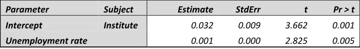
The unemployment rate covariance parameter for the random effects in the model that omits the IMR is significantly different from zero (Table 2). This indicates that the local labour force condition plays a role in labour market outcomes for graduates and module completers. It also adjusts the hierarchical model for this effect.

Table 2 Random effects in employment outcomes (model without IMR)

Parameter Subject Estimate StdErr t Pr > t

Intercept Institute 0.032 0.009 3.662 0.001

Unemployment rate 0.001 0.000 2.825 0.005

Page 6 _of 10

Individual institutions’ results can be found in table 3 (due to space limitations, we only present a subset of all institutions analysed). The institutional estimates can be interpreted as a measure of the difference from the overall mean post training employment rate, after all the confounders have been taken into account. Green shading signifies that the institutional performance in respect to post training employment features significantly above the mean of all providers. Red shading indicates below average performance.

Table 3 Institutional Employment estimates and raw v modelled score comparison (subset only)

Institute Estimate StdErr t P>|t| raw modelled Difference

1 -0.135 0.091 -1.5 0.135 -2% -3% -1%

2 -0.059 0.105 -0.56 0.573 -4% -1% 3%

3 -0.010 0.129 -0.08 0.936 -4% 0% 4%

4 -0.275 0.103 -2.66 0.008 -10% -7% 3%

5 -0.114 0.085 -1.33 0.183 -5% -3% 2%

6 -0.119 0.100 -1.19 0.233 -3% -3% 0%

7 0.032 0.117 0.27 0.784 0% 1% 1%

8 -0.404 0.085 -4.75 <.0001 -16% -10% 6%

10 -0.182 0.074 -2.45 0.014 -6% -4% 2%

11 -0.129 0.112 -1.16 0.247 -2% -3% -1%

12 -0.096 0.089 -1.08 0.280 -7% -2% 5%

13 0.144 0.082 1.75 0.081 2% 4% 1%

14 0.002 0.112 0.02 0.986 2% 0% -2%

15 0.165 0.092 1.79 0.073 4% 4% 0%

16 0.086 0.110 0.79 0.432 7% 2% -5%

17 -0.002 0.117 -0.02 0.985 4% 0% -4%

18 -0.010 0.101 -0.1 0.921 5% 0% -5%

19 0.242 0.113 2.15 0.032 7% 6% -1%

20 -0.082 0.079 -1.04 0.298 -1% -2% -1%

22 0.014 0.090 0.16 0.873 0% 0% 1%

23 -0.104 0.090 -1.16 0.245 -2% -3% 0%

24 -0.166 0.093 -1.78 0.074 -2% -4% -2%

25 -0.006 0.118 -0.05 0.961 6% 0% -6%

26 -0.096 0.127 -0.75 0.451 1% -2% -4%

27 0.045 0.077 0.58 0.563 2% 1% -1%

28 0.141 0.119 1.19 0.234 5% 3% -1%

29 -0.195 0.088 -2.22 0.027 -8% -5% 3%

30 0.267 0.107 2.51 0.012 5% 7% 1%

Page 7 _of 10

exceeds 5% in respect to the average score. This underlines the necessity to employ a well fitting model over a simple calculation of raw scores to construct such performance indicators.

Discussion

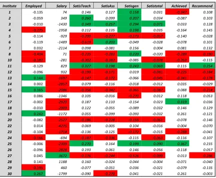
In addition to the employment indicator described in detail above, we have developed and calculated an additional seven indicators from the SOS as mentioned in the introduction. The analysis revealed that the indicators for salaries, satisfaction with teaching, overall satisfaction, perception of achievement, and willingness to recommend contained significant selection bias. We adjusted these models accordingly by incorporating the inverse Mills ratio into the respective models. Table 4 displays all seven indicators by institution, along with their respective shading indicating above or below average performance.

Table 4 Summary of all seven modelled performance indicators (subset only)

Institute Employed Salary SatisTeach SatisAss Satisgen Satistotal Achieved Recommend

1 -0.135 74 0.146 0.127 0.158 0.031 -0.347 0.108

2 -0.059 349 0.260 0.099 0.207 0.034 -0.087 0.103

3 -0.010 -1430 0.349 0.257 0.294 0.071 0.033 0.128

4 -0.275 -1958 0.112 0.135 0.198 0.035 -0.164 0.145

5 -0.114 -929 -0.200 -0.277 -0.173 -0.057 -0.140 -0.028

6 -0.119 -1489 -0.619 0.203 -0.049 -0.028 -0.078 0.101

7 0.032 -2114 0.098 -0.081 0.156 0.004 0.081 0.132

8 -0.404 71 -0.235 -0.283 0.220 -0.020 -0.289 -0.190

10 -0.182 -281 -0.302 -0.382 -0.085 -0.078 -0.263 -0.115

11 -0.129 829 0.327 0.198 0.243 0.069 0.115 0.254

12 -0.096 932 -0.199 -0.171 0.019 -0.081 -0.225 -0.184

13 0.144 -1697 -0.147 -0.172 -0.066 -0.045 -0.341 -0.178

14 0.002 -2857 0.079 -0.116 -0.018 -0.012 0.035 -0.029

15 0.165 -2086 -0.356 -0.342 -0.365 -0.087 0.088 -0.214

16 0.086 -1346 0.105 -0.016 -0.270 0.012 0.118 0.053

17 -0.002 -2920 0.187 0.110 -0.154 0.023 0.319 0.036

18 -0.010 -2009 0.122 -0.055 -0.089 0.032 0.146 0.129

19 0.242 -1172 0.055 -0.099 -0.093 -0.032 0.261 -0.121

20 -0.082 -2527 -0.186 -0.228 -0.155 -0.061 -0.078 -0.146

22 0.014 -4275 0.069 0.005 0.104 -0.016 0.004 -0.070

23 -0.104 -1714 -0.136 -0.125 -0.172 -0.015 -0.288 -0.041

24 -0.166 -694 -0.187 -0.336 -0.115 -0.063 -0.116 -0.107

25 -0.006 -2309 0.270 0.164 0.199 0.090 0.367 0.235

26 -0.096 -2828 0.193 0.061 0.146 0.056 -0.118 0.057

27 0.045 3672 -0.176 -0.244 -0.526 -0.099 0.013 -0.286

28 0.141 1188 0.160 -0.024 0.044 -0.004 -0.071 -0.040

29 -0.195 460 -0.077 -0.051 0.036 -0.021 -0.079 -0.135

30 0.267 -1799 -0.090 -0.270 0.041 -0.021 0.261 -0.003

Page 8 _of 10

employment performance indicator for the prevailing employment conditions in the residential area of students.

From table 4 we can also infer how our performance indicators relate to each other. Table 5 displays the correlations between all eight indicators. In this table we shaded those indicator pairs where the correlation exceeds 0.5.

Table 5 Correlations between modelled performance indicators

Employed Salary SatisTeach SatisAssess SatisGen SatisOverall Achieved Recomm

Employed 1

Salary 0.17 1

SatisTeach 0.19 -0.07 1

SatisAssess 0.16 0.16 0.73 1

SatisGen -0.24 -0.07 0.47 0.53 1

SatisOverall 0.18 -0.01 0.84 0.82 0.59 1

Achieved 0.58 0.21 0.23 0.26 0.01 0.34 1

Recommend 0.24 -0.07 0.60 0.61 0.33 0.77 0.31 1

Not surprisingly, all three types of student satisfaction correlate with overall satisfaction. Overall satisfaction also correlates with the ‘recommend’ indicator. ‘Willingness to recommend’ their institution correlates strongly with ‘satisfaction with teaching’ and ‘assessment’, and ‘overall satisfaction’, and less so with ‘general learning satisfaction’. Employment correlates highly with ‘achievement’ indicating that students consider positive employment outcomes as the main marker for achievement.

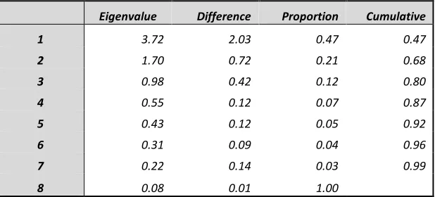
In order to assess if our performance indicators could be abstracted into coherent groups, we performed a principal component analysis of all seven modelled indicators. The Eigenvalues of the correlation matrix can be found in table 6.

Table 6 Eigenvalues of the correlation matrix of 7 performance indicators

Eigenvalue Difference Proportion Cumulative

1 3.72 2.03 0.47 0.47

2 1.70 0.72 0.21 0.68

3 0.98 0.42 0.12 0.80

4 0.55 0.12 0.07 0.87

5 0.43 0.12 0.05 0.92

6 0.31 0.09 0.04 0.96

7 0.22 0.14 0.03 0.99

8 0.08 0.01 1.00

Page 9 _of 10

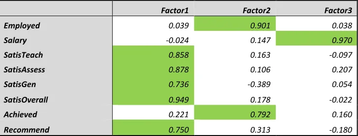
of the original variance. The rotated factor pattern is displayed in table7. Highly associated items are shaded in green.

Table 7 Rotated factor pattern for 3 factor solution

Factor1 Factor2 Factor3

Employed 0.039 0.901 0.038

Salary -0.024 0.147 0.970

SatisTeach 0.858 0.163 -0.097

SatisAssess 0.878 0.106 0.207

SatisGen 0.736 -0.389 0.054

SatisOverall 0.949 0.178 -0.022

Achieved 0.221 0.792 0.160

Recommend 0.750 0.313 -0.180

It can be seen that all satisfaction items plus the willingness to recommend the institution fall into one dimension (e.g. measure a similar concept). The second dimension consists of the probability of being employed and sense of achievement. Finally, salary outcomes are a distinct performance measure that is unrelated to any other performance indicator.

We should note that, as in any study, there are some limitations to this analysis that should be kept in mind when interpreting the results.

Firstly, the models employed here obviously capture only those covariates that we were able to observe. In particular, the models relating to student satisfaction have, while statistically significant, only limited explanatory power. This means that there are other effects that impact on student satisfaction which we did not capture within the Student Outcomes Survey.

A second limitation is the limited response rate to the SOS, which is in the area of 35 percent. This issue is further magnified in the model analysing post training salaries, as only a third of SOS respondents answers the salary question.

Finally, as in most surveys, there is some inherent respondent bias in the SOS. This is often caused by higher (or lower) response rates of particular groups (for instance, males are often less likely to return a response than females). While we have attempted in this analysis to employ corrective measures that aim to alleviate (non-) response bias, the possibility cannot be excluded that some residual survey bias exists.

Conclusion

Page 10 _of 10

graduate/module completer status, labour force status prior to training, and employment and wage conditions in the area of student’s residence.

The resulting institutional comparison table gives a clear picture of how each respective institute scores in regard to individual performance indicators. Those that score significantly below or above the national average can be easily visualised via a shading scheme.

A further important finding is that the modelled performance indicators proposed in this paper appear to have a significant advantage over simple (raw) indicators. Modelled performance indicators enable us to compare institutions on a more even footing as we are adjusting for the most important demographic and environmental variables. As a result we can see that while the correlation between raw and modelled performance indicators is quite strong, there are significant differences between the scores of individual institutions.

Finally, we found that the proposed eight performance indicators could be categorised into several coherent groups: In our present case possible groupings may be student satisfaction and willingness to recommend, achievement and employment outcomes, and post training salary.

Bibliography

Dai, J., Li, Z., & Rocke, D. (2006). Hierarchical logistic regression modeling with SAS GLIMMIX. In Conference Proceedings of Western Users of SAS Software (pp. 27-29).

Dubin, J. A., & Rivers, D. (1989). Selection bias in linear regression, logit and probit models. Sociological Methods & Research, 18(2-3), 360-390.

Fieger, P. (2012). Measuring student satisfaction from the Student Outcome Survey, National Centre for Vocational Education Research, Adelaide, 2012

Heckman, J. J. (1979). Sample selection bias as a specification error. Econometrica: Journal of the econometric society, 153-161.

Karmel, T., & Fieger, P. (2012). The value of completing a VET qualification, National Centre for Vocational Education Research, Adelaide, 2012

Labour market data. (2011).

Http://foi.deewr.gov.au/system/files/doc/other/australian_regional_labour_markets_september _quarter_2011.pdf

Technical SOS description. (2012).

http://www.ncver.edu.au/statistics/surveys/sos12/sos12_Technical_notes.pdf

Transparency agenda. (2012).