Munich Personal RePEc Archive
Identifying observed factors in
approximate factor models: estimation
and hypothesis testing
Chen, Liang
Universidad Carlos III de Madrid
20 March 2012
Online at
https://mpra.ub.uni-muenchen.de/37514/
Identifying Observed Factors in Approximate Factor Models:
Estimation and Hypothesis Testing
Liang Chen Universidad Carlos III de Madrid
(This version: March, 2012)
Abstract
Despite their popularities in recent years, factor models have long been criticized for the lack of identification. Even when a large number of variables are available, the factors can only be consistently estimated up to a rotation. In this paper, we try to identify the underlying factors by associating them to a set of observed variables, and thus give interpretations to the orthogonal factors estimated by the method of Principal Components. We first propose a estimation proce-dure to select a set of observed variables, and then test the hypothesis that true factors are exact linear combinations of the selected variables. Our estimation method is shown to able to cor-rectly identity the true observed factor even in the presence of mild measurement errors, and our test statistics are shown to be more general than those of Bai and Ng (2006). The applicability of our methods in finite samples and the advantages of our tests are confirmed by simulations. Our methods are also applied to the returns of portfolios to identify the underlying risk factors. Keywords: Factor Models, Observed Factors, Estimation, Hypothesis Testing
1. Introduction
Factor models (FM henceforth) are becoming an increasingly important tool for both theo-retical and empirical research. For example, in macroeconomics, the solutions of DSGE models can be written in the form of FM when these models allow for measurement errors (Altug 1989 and Sargent 1989 ), so that the structure of FM can help solve these models even when a large number of variables are considered (Boivin and Giannoni 2006, Kryshko 2011); in structural analysis, the factors estimated from large panel datasets can be combined with Structural Vector Autoregressions (SVAR) to identify the effects of fundamental shocks (Bernanke et al 2005), and solve the problem ofnon-fundamentalness(Forni et al 2009). Moreover, the estimated factors can significantly improve the forecasts of macro variables (Stock and Watson 2002a). In mi-croeconomics, the demand systems are shown to have a factor structure (Lewbel 1991), and in some recent studies, FM are used to characterize the unobservable cross-sectional dependencies in panel data models (Pesaran 2006 and Bai 2009). Finally, in finance, the key assumption under-lying the Arbitrage Pricing Theory (APT) is the multi-factors structure for the security returns.
from the restrictive assumptions of the classical factor analysis, and estimate the factor models consistently using the method of Principal Components (PC hereafter) (Bai and Ng 2002, Bai 2003, Stock and Watson 2002a).
Yet, it is well recognized that FM suffer from identification problems. Consider a factor model: xt = Λft+et, where xt is the vector of observed variables, Λis the matrix of factor
loadings,ftis the unobservable factors, andetis the vector of idiosyncratic errors. Since only xtcan be observed, the above model is observably equivalent to: xt =(ΛH−1)(Hft)+et, where His anyr×rnonsingular matrix. Therefore, unless one imposesr×r prior restrictions, the factors can only be identified up to a rotation, and thus the estimated factors usually lack a direct interpretation.1.
In some situations, the object of interest is the conditional mean of some observed variables, so that the interpretation of the factors is not important. For example, in panel data models, one only needs to consistently estimate the common parts (Λft) of the unobservable effects, and thus
the indeterminacy of the factors rotation does not matter for the results.
However, there are other instances where the direct object of interest are the factors them-selves and thus a clear interpretation of them can have important implications for structural anal-ysis. In financial economics, a large body of empirical research is concerned with identifying the factors that determine the prices of the securities. Chen et al (1986) and Shanken and We-instein (2006) are examples of such work that try to interpret the underlying forces in the stock market in terms of some observed macro variables. Instead of using macro variables, Fama and French (1993) identify three observed factors related to the market returns and firm characteris-tics, which can explain most volatilities of the assets returns. In the solutions of DSGE models, the state variables and exogenous shocks (e.g., preference shocks or technology shocks) play the role of common factors, so that the interpretation of the factors is equivalent to identifying the sources of business cycles. In factor-based forecasts, not all the estimated factors necessarily have prediction power for the target variables (Tu and Lee 2011), and hence the forecasting can be further improved if some interpretational contents are attached to the factors. For example, the predictions of inflation rates could be more accurate if the factors associated with monetary policy shocks are given more weight than other factors identified as productivity changes (For more examples see Bai and Ng, 2006).
The goal of this paper is to identify the factors by relating them to some observed variables. The point of departure is the assumption that the common factors can be well approximated by (or linear functions of) some observed variables. Under this assumption, we will denote these observed variables asobserved factors. We focus on the approximate factor models (Chamber-lain and Rothschild 1983, Bai and Ng 2002) which allow for quite general assumptions about the data generating processes (DGP henceforth). More importantly, the space of the factors can be consistently estimated using the method of PC under the assumption of largeN (the number of variables).
To the best of our knowledge, Bai and Ng (2006) is the only work that has addressed this issue.2. These authors consider the null hypothesis: gt = Lft for am×rmatrix Land a list
of m(> r) observed variablesgt, suggested by some economic reasoning. They develop test
1The conventionally adopted identification assumptions for the estimation of factors using PC are that: (i) the factors
are orthogonal and (ii) the covariance matrix of the factor loadings is diagonal.
2Bai and Ng (2011) study the identification of factors from a statistical point of view, i.e., by imposing restrictive
assumptions on the data generating processes of the factors and factor loadings.
statistics for each of the observed variablesgktas well as for the whole set of variablesgt, based
on the regressions ofgton the estimated factors.
In practice, however, the list of observed factors is not always available, or those suggested by economic theory may not span the same space of the underlying factors. In view of these caveats, we propose here to firstestimate(in the precise sense defined below) a list of observed factors from a much larger set of variables, and then test the null hypothesis that the underlying factors are exact linear combinations of observed variables selected in the first step.
In the estimation part, the estimated factors are regressed on different subsets of observed variables, and we label as theestimated observed factors that subset of variables that mini-mizes the Residual Sum of Squares (RSS) in these regressions. We differentiate two cases of observed factors: thedirectly observed factors (DOFs henceforth) and theindirectly observed factors(IOFs). In the first case, the latent factors in the FMs are directly approximated by the observed factors, i.e., there is a one-to-one correspondence between therfactors androbserved variables. In the second case, by contrast, therfactors are linear functions ofmobserved vari-ables withm≥r. Notice that this second setup includes the first one as a special case, but we will show that, for DOFs, our estimation method is much simpler and allows for larger measurement errors (i.e., the difference between the latent factors and the observed factors).
In the testing procedure, we consider the null hypothesis: ft =Bx1:m,tfor ar×mmatrixB
and a list ofmobserved variablesx1:m,t. This hypothesis covers both cases discussed above, and
is shown to be more general than the hypothesis considered by Bai and Ng (2006). We derive two types of test statistics based on the residuals in the regressions of estimated factors onx1:m,t.
The advantages of our tests are that: (i) each of the proposed tests can be viewed as a test for the whole set ofx1:m,t, rather than each element ofx1:m,t; (ii) though Bai and Ng (2006) also proposed
a test for the whole set ofx1:m,t, our tests are derived under less restrictive conditions; (iii) since
we consider a more general hypothesis, the tests of Bai and Ng (2006) tend to reject the null in the case of IOFs, while our tests still perform well.
The rest of the paper is organized as follows: Section 2 defines the basic notations and dis-cusses the assumptions that define the approximate factor models. In section 3 we define the directly observed factors, and show how to identify them through estimation. The definition and identification ofindirectly observedfactorsare analyzed in Section 4, where we also discuss how to implement the method in practice. In section 5, we define the null hypothesis of observed factors and propose several test statistics whose asymptotic distributions are also derived. Sec-tion 6 studies the finite sample properties of the estimaSec-tion methods and the test statistics, paying particular attention to their performance relative to the tests of Bai and Ng (2006). In Section 7 we apply our method to identify the risk factors for the returns of portfolios. Finally, Section 8 concludes. All the proofs are collected in the Appendices.
2. Models, Notations and Assumptions
Throughout this paper, we use the following standard notation. We define the matrix norm: ∥A∥ = √Tr(A′A), and useA1:m to denote the 1st tom−th rows of a matrix (or a vector) A.
Further,A>0 (≥0) means that the matrixAis positive (semi) definite. The following approximate factor models are considered:
xt=Λft+et, (1)
wherext =(x1t, . . . ,xNt)′is a N×1 vector of observed variables,Λ =(λ1, . . . , λN)′is a N× rvector of factor loadings, ft = (f1t, . . . ,frt)′ is ar×1 vector of common factors, andet =
(e1t, . . . ,eNt)′is aN×1 vector of idiosyncratic errors. Unlike the classical factor analysis, we
allow the number of variablesNto go to infinity and the errors{eit}to be both temporarily and
cross-sectionally correlated.
We assume thatmamong the observed variablesxt areobserved factors, in a sense to be
defined in the following sections, wheremis a fixed number that does not increase asNgoes to infinity. Without loss of generality, we assume thesem observed factorsare ordered as the first mvariables ofxt. The main issue is how to find the thesemobserved variables in the available
set of size N . Given that them observed factors are always placed in the firstmrows, this issue becomes equivalent to finding out the firstmvariables out ofNrandomly ordered observed variablesxt.
We consider two cases: DOFs and IOFs. In either case, themobserved factors have the following form:
x1:m,t=Λ1:mft+e1:m,t. (2)
To single out the observed factors, we have to impose some restrictions onΛ1:mande1:m,t, which
will be discussed in Sections 3 and 4. Roughly speaking, for the DOFs,Λ1:mshould be a
full-rank matrix ande1:m,tshould go to zero asNandTgo to infinity; for IOFs, a necessary condition
is that the covariance matrix ofe1:m,thas reduced rank.
Next we impose some assumptions forΛ,ftandet. The following assumptions are necessary
for the consistency of estimated factors using PC. Further, it should be noted that the assumptions to be imposed in Sections 3 and 4, when defining the observed factors, do not contradict with the following ones.
LetMdenote a finite constant, we assume that:
Assumption 1. (i) E||ft||4 < M for t = 1, . . . ,T , and T1 ∑1Tftft′ → ΣF > 0as N,T → ∞; (ii) E||λi||4 <M for i=1, . . . ,N, and N1 ∑1Nλiλ′i →ΣΛ>0as N,T → ∞; (iii) The r eigenvalues of
ΣΛΣFare different.
Assumption 2. (i) E(eit)=0, E(eit)8≤M;
(ii) For i,j = 1, . . . ,N and s,t = 1, . . . ,T , E(eitejs) = τi j,ts, |τi j,ts| ≤ τi j for all (t,s), and
|τi j,ts| ≤γtsfor all(i,j). N1 ∑i,jτi j ≤M,T1 ∑t,sγts≤M, NT1 ∑i,j,t,s|τi j,st| ≤M, and∑sγ2st ≤M; (iii) For any(t,s), E|N−1/2∑N
i=1[eiseit−E(eiseit)]|4≤M. Assumption 3. {λi},{ft}and{eit}are three independent groups.
These Assumptions are quite general in the sense that they allow heteroskedasticitiy, temporal and cross-sectional correlations in the factors and idiosyncratic terms. For more discussion on these Assumptions, see Bai (2003). Under Assumptions 1 to 3, the Information Criteria (IC) proposed by Bai and Ng (2002) can consistently estimate the number of factors, so that we can proceed as if this number was known. The effect of misspecification of the factor numbers is discussed in Section 4.
Define theT ×rmatrix ˜F=(˜f1, . . . ,˜fT)′as
√
T times the eigenvectors corresponding to the rlargest eigenvalues of theT ×T matrixXX′, where theT ×NmatrixX=(x
1, . . . ,xT)′. Then,
denoting min[√N,√T] asδN,T, the following result holds:
Lemma 1. (Bai and Ng 2002) Under Assumptions 1 to 3,δN,T||˜ft−H′ft||=Op(1)for t=1, . . . ,T , whereH=(Λ′Λ
N
)(F′F˜ T
)V−1
NT, andVNT is a diagonal matrix containing the r largest eigenvalues of
(NT)−1XX′.
Lemma 1 is a key result underlying our identification method for observed factors. It implies that the estimated factors are consistent for the space spanned by the true factors and hence for the observed factors. This relationship between the estimated factors and observed factors can be explored to identify the latter. For the identification of IOFs, the convergence rateδN,T is
important to design an appropriate objection function, as will be shown in Section 4.
However, it is worth stressing that we do not consider aweak factorsstructure as in Onatski (2009a), in which the PC estimator of the factors are not consistent if their explanatory power is small relative to the idiosyncratic terms. In our setup, factors are strong whenver Assumption 1 is satisfied.
3. Directly Observed Factos
In this section, we deal with the identification of the DOFs. To give the precise definition of DOFs, the following assumptions are made:
Assumption 4. (i) m=r,Λ1:rhas full rank, and eit=κN,Tεitfor i=1, . . . ,r, whereκN,T →0as N,T → ∞;
(ii)εt=(ε1t, . . . , εrt)′, T1∑tT=1εtε′t→Σεand||Σε|| ≤M;
(iii) LeteN1:Nr,t=(eN1,t, . . . ,eNr,t)′for r+1≤N1<N2. . . <Nr≤N, then
1 T
∑T
t=1eN1:Nr,te′N1:Nr,t→
Σe
N1:Nr >0.
Assumption 4(i) states that the first r variables span the space of the common factors ft
asymptotically: x1:r,t → Λ1:rftas N,T → ∞. WhenΛ1:r = Ir, it simply means the common
factors are directly measured by the firstr observed variables with neglectable measurement errors. Notice that the nonsingular matrixΛ1:r is just a normalization, and hence we can define
the new factors asgt =Λ1:rft which are directly measured byx1:r,t, because for the remaining
variables we have:
xm+1:N,t = Λm+1:Nft+em+1:N,t
= (
Λm+1:NΛ−1:r1
)(
Λ1:rft)+em+1:N,t
= Λ∗m+1:Ngt+em+1:N,t
Therefore, we label the firstrobserved variablesDirectly Observed Factors. Notice Bai and Ng (2006) identify the observed factors by constructing some test statistics under the assumption of an exact relationship between the observed variables and the factors, i.e.,e1:r,t = 0 fort =
1, . . . ,T. By contrast, we allow for small measurement errors in the case of DOFs. We will show that the larger these measurement errors, the more difficult is the identification of the DOFs. Indeed, whenκN,T =1, there is no differences between the firstmvariables and the remaining N−mones.
Assumption 4(iii) rules out (asymptotic) multi-collinearity between any set of r observed variables, such thatT1∑T
t=1xN1:Nr,tx′N1:Nr,t→Σ
x
N1:Nr >0 for 1≤N1< . . . <Nr ≤N.
From Lemma 1 and Assumption 4 we can derive an approximate linear relationship between the estimated factors and the DOFs:
˜
ft=Hft+op(1)=HΛ−1:r1x1:rt+op(1)=Ax1:r,t+op(1), (3)
whereA=HΛ−1
1:r. As will be defined shortly, our method of identification is based on the
regres-sions of therestimated factors onrobserved variables (in contrast to Bai and Ng 2006 where the observed variables are regressed on the estimated factors). The intuition for our approach is that, if ˜ftare regressed on the right set of observed variables: x1:m,t, the OLS estimator ˆAwill
converge toAand the residuals will beop(1), so that RSS/Twill converge to 0. If the regressors
are chosen as a set ofrobserved variables different fromx1:r,t, we show that RSS/T will instead
converge to some positive numbers. As a result, we can identify the DOFs by comparing the RSS in the regression of ˜fton different sets of observed variables.
LetN1:Nr=[N1, . . . ,Nr] denote a set ofrindices such that 1≤N1<N2 < . . .Nr≤N, and
letxN1:Nr,t=ΛN1:Nrft+eN1:Nr,tbe the corresponding observed variables. By defining:
S(N1:Nr,A)=
1 T
T
∑
t=1
˜
ft−AxN1:Nr,t
2 , (4) and
[ ˆN1,Nˆ2, . . . ,Nˆr]=arg min N1:Nr
(
min
A S(N1 :Nr,A)
)
, (5)
thenxNˆ1: ˆNr,tis the vector of DOFs identified by our method.
Notice that
1 T
T
∑
t=1
˜
ft−AxN1:Nr,t
2 = 1 T r ∑
k=1 T
∑
t=1
(
˜
fkt−a′kxN1:Nr,t
)2
,
and therefore
min
A S(N1:Nr,A)=S(N1:Nr,
ˆ
A),
where ˆA′ = [ˆa1,aˆ2, . . . ,aˆr], and ˆakis the OLS estimator ofak. This procedure can be simply
implemented as follows: we first chooserobserved variables, then calculate RSSkin the OLS
regression of ˜fkton these chosen variables, and get RSS=∑rk=1RSSk, where the set of variables
that yield the smallest RSS are the identified DOFs.
The following theorem states that, using our method, the probability of correctly identifying the DOFs goes to 1 asNandT go to infinity.
Theorem 1. Under Assumption 1 to 4,P([ ˆN1,Nˆ2, . . . ,Nˆr]=[1,2, . . . ,r]
)
→1as N,T → ∞. This result holds as long asκN,T =o(1). However, with finite samples, the DOFs may not be
easily distinguishable from the remaining variables, due to either large measurement errors (κN,T)
or large estimation errors of the PC. The finite sample properties of our identification procedure will be studied in Section 5 using simulations.
4. Indirectly Observed Factors
4.1. Definitions and comparison with Bai and Ng (2006)
In the previous section, we have studied the simple case where the common factors are di-rectly observed, i.e.,ft =x1:r,t fort = 1, . . . ,T. However, in practice it is quite likely that the
common factors are well approximated by the linear combinations of some observed variables, i.e.,ft=Bx1:m,tfor ar×mmatrixBwith full row rank. For example, one of the macro variables
considered by Chen et al (1986) is the spread of interest rates. Whenm=r, we have shown in the previous section that this case is equivalent to DOFs. Further, whenm<r, the space spanned by the factors has rankm,instead ofr, and so we should getmfactors using Bai and Ng’s IC. Hence, without loss of generality, we focus on the case:m>rthroughout this section.
We impose the following assumption to define the IOFs:
Assumption 5. (i)ft =Bx1:m,tfor t=1, . . . ,T , the r×m matrixB=(b1, . . . ,bm)has full row rank, and∥bk∥2,0for k=1, . . . ,m;
(ii) x1:m,t = Λ1:mft +e1:m,t, and e1:m,t = C1ϵt, where C1 is a m×(m−r) matrix such that C=[Λ1:m,C1]is a full rank matrix.
(iii) For any constant number k, and any set of indices1≤N1< . . . <Nk≤N,T1
∑T
t=1xN1:Nkx′N1:Nk
p
→ Σx
N1:Nk >0.
(iv) For any set of k indices: m+1≤N1< . . . <Nk≤N,T1∑Tt=1eN1:Nk,te′N1:Nk,t
p
→Σe
N1:Nk >0.
Although Assumption 5(ii) implies that the relation ft = Bx1:m,t does exist, Assumptions
5 (i) (iii) and (iiii) guarantee that the IOFsx1:m,t are uniquely determined. To see this notice
that, from Assumption 5(ii), we can writex1:m,t =C
(
ft
ϵt
)
. It follows thatC−1
1:rx1:m,t =ft, which
yields the expression in 5(i) withB=C−1
1:r. Yet, Assumption 5(ii) alone is not enough to define
a unique set of IOFs. For example, whenC = I, we haveC−1
1:r = (Ir,0), and thusft = x1:r,t,
which reduces to the case of DOFs. Besides, ifx1:m,t are IOFs,x1:m+1,twill also be IOFs, since ft =(B,0)x1:m+1,t. Therefore, the second part of Assumption 5(i) is necessary to exclude these
undesirable cases. Moreover, Assumption 5(iii) excludes multi-collinearity among the element of any subset of observed variables. Together with 5(iv), it rules out the existence of IOFs formed by linear functions of other variables.
Note that the assumptionft = Bx1:m,t is essential. To see this, recall that the hypothesis of
interest in Bai an Ng (2006) is thatgt =Lft for am×rmatrixL,so that their tests are based
on the regressions of the observed variables:gton the estimated factors: ˜ft. On the contrary, as
mentioned above, we regress the estimated factors on the observed variables. The difference is trivial for the case of DOFs since, given that the observed variables span the same space of the factors and that the estimated factors are consistent for the true factor space, then both regressions will produce neglectable residuals. However, this difference becomes nontrivial for the case of IOFs.
We use a simple example to illustrate the difference for IOFs. Consider a factor model with only one factor: ft=x1t−x2tfort=1, . . . ,T, wherex1tandx2tare two observed variables. The
null hypothesis considered by Bai and Ng (2006) is:
(
x1t x2t
)
=
(
c c−1
)
ft, (6)
wherecis any real number. Suppose now there is an estimator ˜ftsuch that ft = f˜t+op(1), one
can write
x1t=cf˜t+op(1), (7)
and the residuals in the regression ofx1ton ˜ftwill beop(1) (note that the result is similar forx2t).
Their test statistics are based on exploring the exact order of theop(1) term, namelyOp(1/
√ N) when √N/T →0. Now suppose there is another observed variable:x3t= ft+e3twith Var(e3t)=
σ2>0.Then, since the residuals in the regression ofx3ton ˜ftwill be larger thanop(1) because
we can writex3t= f˜t+e3t+op(1),their tests have power to rejectx3tas a member ofgt.
In our definition, only ft = x1t−x2tis required, whereas x1tand x2tare allowed have the
following FM representation:
(
x1t x2t
)
=
(
c c−1
)
ft+
(
1 1
)
εt, (8)
for any real numbercand random processεt. Note that (6) is a special case of (8) withεt =0
but withx1tandx2tbeing defined as in (8), the tests of Bai and Ng (2006) will reject the null if
εtis a process with positive variance, despite being true that ft=x1t−x2t.
To summarize, the null hypothesis considered by Bai and Ng (2006) is equivalent to the definition of DOFs without measurement errors. Hence,it is less general the definition of IOFs considered here.
4.2. Identifying the IOFs
The idea for identifying the IOFs is similar to the identification of DOFs. If the number of IOFs:mis a priori known, one can use the method in Section 3 to select themoutNobserved variables that yield the smallest RSS, where the probability of correctly selecting themIOFs goes to 1 asNandT goes to infinity.
However, whenmis not known in practice, one is faced with the choices of bothmandx1:m,t.
Let ˆmbe an estimator ofm. If ˆm<m, then any ˆmselected variables cannot span the space of the rfactors, since otherwise Assumption 5(i) will be violated. Then the sum of RSSs (divided byT) in the regressions of the estimated factors on the selected observed variables will be positive. If
ˆ
m=m, the sum of RSSs (divided byT) will converge to 0 ifx1:m,tare selected. However, when
ˆ
m > mandx1:m,t are among the selected variables, the sum of RSSs (divided byT) will also
converge to 0 because adding more regressors never increases the RSSs. To solve this problem, we need to impose some penalty functions for adding extra regressors.
To do so, let us define:
[ ˆm,Nˆ1,Nˆ2, . . . ,Nˆmˆ]= arg min r≤k≤kmax,N1:Nk
(
S(N1:Nk,Aˆ)+k·p(N,T)
)
, (9)
whereS(N1 :Nk,Aˆ) is as defined in Section 3,kmaxis a predetermined constant, andp(N,T) is
a penalty function depending onNandT. The following theorem constitutes the main result of this paper:
Theorem 2. Under Assumptions 1, 2, 3 and 5,
P[ ˆm=m,( ˆN1, . . . ,Nˆmˆ)=(1, . . . ,m)]→1
as N,T → ∞, if kmax≥m, p(N,T)→0andδ2N,Tp(N,T)→ ∞as N,T → ∞.
The estimation procedure in Section 3 is repeated for different values ofk, and we add a penalty term to the object function. Theorem 2 implies that one can identify the number of IOFs and the IOFs simultaneously with probability approaching to 1 as N and T increase.
4.3. The choice of penalty functions
Since the penalty functions in our procedure and those considered by Bai and Ng (2002) have to satisfy the same conditions, we can use some of their choices that have been proved successful in determining the number of factors. Particularly, we consider the following three penalty functions:
p1(N,T)=
(
N+T NT
)
ln
(
NT N+T
)
,
p2(N,T)=
(
N+T NT
)
ln(δ2 N,T
),
p3(N,T)=
lnδ2 N,T
δ2N,T .
These penalty functions have the same asymptotic properties but may perform differently in finite samples ( see Bai and Ng, 2002) for a detailed discussion). The finite sample properties of our method using these functions are studied in the Section 6.
4.4. Practical implementation
In the previous discussion, we have assumed that the number of factors (r) is known or cor-rectly estimated. However, in practice, the estimated number of factors using different methods usually differ for the same data set. For example, if one applies the test of Onatski (2009b) to the U.S macro data set used in Stock and Watson (2009), 2 factors can be found; but if one uses the 6 different information criteria of Bai and Ng (2002) to the same data, the estimated numbers of factors range from 2 to 6. Actually, it is very rare in practice that the number of factors can be uniquely determined by different methods. Therefore, a discussion on how to implement our methods in practice becomes necessary when the number of factors cannot be correctly specified.
When the estimated number of factors ˆris larger than the true oner, Lemma 1 does not hold, so that the above-mentioned methods will fail to identify the IOFs (or DOFs). When ˆr < r, Lemma 1 continues to hold, but our methods will not necessarily identify all of the IOFs. To see this, we first write:
˜
ft=H′Bx1:m,t+op(1)=Ax1:m,t+op(1)
by Lemma 1 and Assumption 5(i), where the matrixA=H′Bisr×m. Leta
kbe thekth row of A, then ˜fkt =akx1:m,t+op(1). If we apply our procedure to each of the ˜fktfork=1, . . . ,r, then
˜
fktcan only identify those variables corresponding to the non-zero elements of ¯ak=plimak. For
example, ifa1 p
→ (1,0, . . . ,0), ˜f1t can only identifyx1t. However, Theorem 2 guarantees that
the union of the variables identified by ˜f1tto ˜frtis equal to the IOFs. The reason is that, sinceH
(also plimH) is nonsingular andBhas no zero columns (Assumption 5(i)),A(also plimA) does not have zero columns.
The previous discussion suggests that we can implement our procedure as follows: Instead of regressing all the estimated factors on the observed variables, we run the regression for each of the estimated factors, starting with the first one: ˜f1t. For each ˜fkt, define:
[ ˆmk,Nˆ1,Nˆ2, . . . ,Nˆmˆk]= arg min
r≤h≤kmax,N1:Nh
(1
T T
∑
t=1
( ˜fkt−aˆkxN1:Nh,t)
2+h
·p(N,T)), (10)
where ˆak is the OLS estimator and p(N,T) is as defined above. The key here is when to stop
the process. If one stops whenk<r, the union of the selected variables may be a subset of the IOFs; if one stops whenk>r, some of the selected variables will not belong to the IOFs. The practitioner can combine the results with some economic theory to judge the appropriateness of the selected variables. If some obvious irrelevant variables are selected for some largek, one should stop the process and restrict attention to the variables already selected.
The main advantage of this procedure is that one can at least identify all of the IOFs, at the cost of identifying some non-IOF variables. While the result in Theorem 2 is much simpler, one bears the risk that none of the selected variables belong to the IOFs when the estimated number of factors is larger thanr.
Another practical issue is that the computational cost of our method tend to explode asN,r, mandkmax increase. As will be shown in the simulations, whenN = 100,r = 2,m = 3 and kmax =4, the searching process takes about 1 hour. 3 In practice,N is at least around 100 in
most cases, and can be as large as thousands in financial data sets. Since the number of factorsr usually ranges from 2 to 8 in many applications, if we were to search in the whole set of variables for those cases, the computational cost could be huge.
To solve this problem, we can restrict our attention to a subset ofnvariables withn < N. Theorems 1 and 2 should still hold if thesenvariables contain the observed factors (DOFs or IOFs). In practice, a list ofn candidate variables can be selected by prior knowledge and/or economic reasoning. In theory, with large samples, our methods should correctly select the observed factors as long as they are contained in then variables. However, in practice, the accuracy of our approach with finite samples will depend onn: the smallern, the less time the computation takes, and the more likely that the observed factors are identified. But a smaller nmeans that one has to exclude more variables and thus it becomes more likely to miss the IOFs. To reach a balance, we should makenas large as possible whenever the computation cost is affordable. The finite sample performances of our methods when selection is restricted ton variables are studied in Section 6.
Another shortcut that can significantly reduce the computation cost is to start the searching process with a large number of regressors,l.In the proof of Theorem 2 (See Appendix B), it is shown that ifl >m, we will select the IOFs (x1:m,t) with otherl−mvariables with probability
approaching 1 asNandT go to infinity. In the next step, we only need to search among thel selected variables in the first step. By a simple conditional probability argument, this modified procedure should have the same asymptotic property as the procedure in (9). The computation cost will be greatly reduced since the second step is really easy to calculate. Moreover, the vari-ables selected in the first step can be combined with other varivari-ables to form a list ofnvariables. In this case the computation cost mainly depends onrmax(the maximum ofl) andN(orn).
3The calculations are implemented with Matlab 2009
5. Hypothesis Testing
So far we have assumed the existence of observed factors. Nevertheless, it is possible that the factors cannot be approximated by any observed variables, such as the potential GDP and the natural rate of unemployment. In such a case, it is necessary to design some tests for the null hypothesisH0 :ft =Bx1:m,t when some observed factors have been selected by our estimation
methods. In this section, we propose several test statistics for theH0 based on both individual
and multiple regressions. Notice that theH0here covers both DOFs and IOFs, because DOFs
can be viewed as a special case of IOFs withBbeing ar×rnonsingular matrix. We differentiate these two cases in the estimation because the method for identifying DOFs is simpler, although the method for identifying IOFs includes DOFs as a special case.
The key result underlying our tests is the following lemma proved by Bai (2003):
Lemma 2. √N(f˜
t−H′ft) d
→N(0,Ωt)if
√
N/T →0as N,T → ∞, whereΩt=V−1QΓtQ′V−1, andΓt=limN→ N1
∑N
i=1
∑N
j=1E(λiλ′jeitejt).
The matricesVandQare defined in Appendix A. It follows that: √
N(f˜
kt−h′kft) d
→N(0, σ2t,k), (11)
wherehkis thekth column ofHandσt2,k=Ωt(k,k). Our tests are based on the residuals in the
regression of the estimated factors on the selected observed variables. Lemma 1 and the null hypothesis imply that ˜ft =H′ft+vt =Ax1:m,t+vt, wherevt =f˜t−H′ft andA=H′B. Let ˆA
denote the OLS estimator ofA, then: ˜
ft=Axˆ 1:m,t+(A−Aˆ)x1:m,t+vt=Axˆ 1:m,t+vˆt,
where ˆvt=(A−Aˆ)x1:m,t+vt. It follows that
√ Nvˆt−
√ Nvt=
√
N(A−Aˆ)x1:m,t. Therefore
√ Nvˆt
should converge to the same distribution of √Nvtbecause
√
N(A−Aˆ)=op(1). To see this, we
can write:
ˆ
A−A=(1 T
T
∑
t=1
x1:m,tx′1:m,t
)−1(1
T T
∑
t=1 x1:m,tv′t
)
.
By Assumption 5,(T1∑T
t=1x1:m,tx′1:m,t
) p
→Σ1:mx >0, and
1 T
T
∑
t=1
x1:m,tv′t=Λ1:m
1 T
T
∑
t=1 ftv′t+
1 T
T
∑
t=1 e1:m,tv′t.
By Lemma B1 and B2 of Bai (2003),T1∑T
t=1ftv′tandT1
∑T
t=1e1:m,tv′tare bothOp(δ−N2,T), whereby it
follows that√N(A−Aˆ)=Op( √
N
min[N,T]), which isop(1) under the condition that
√
N/T →0. As a result of Lemma 2 and the previous analysis, the distribution of the residuals ˆvtin the regressions
of ˜ftonx1:m,tcan be derived as follows:
Nvˆ′tΩ−t1vˆt d
→χ2r, (12)
N
(vˆkt
σt,k
)2 d
→χ21, (13)
where ˆvktis thekth element of ˆvt, i.e., the residuals in the regression of ˜fktonx1:m,t.
Based on these results, we can construct two types of tests. The first type is similar to the A(j) test statistics of Bai and Ng (2006). First, we define:
ˆ
ρt=Nvˆ′tΩˆ− 1
t vˆt, ˆρt,k=N
(vˆkt
ˆ σt,k
)2
, (14)
and
A= 1 T
T
∑
t=1
1( ˆρt>Φr,α) (15)
Ak=
1 T
T
∑
t=1
1( ˆρt,k>Φ1,α) fork=1, . . . ,r. (16)
whereΦr,αandΦ1,αare two constants such thatP[χ2r ≥Φr,α]=P[χ21 ≥Φ1,α] =α, and ˆΩtis a
consistent estimate ofΩt4.
By the results in (12) and (13), E(1
( ˆρt > Φr,α)) = P[ ˆρt > Φr,α] → α. Then, using the
argument behind the Law of Large Numbers (LLN) we can prove the following result:5
Proposition 1. Under Assumptions 1 to 3 and the hypothesis thatft =Bx1:m,tfor t=1, . . . ,T , thenA→p αandAk
p
→αfor k=1, . . . ,r if √N/T →0as N,T → ∞.
Notice once more that theA(j) test of Bai and Ng (2006) is based on individual regressions of the observed variables on the estimated factors (regress each ofx1:m,t on ˜ft), while we do
the opposite here (regress each of ˜ftonx1:m,t). As discussed in Section 4, the advantage of our
procedure is that it allows us to consider more general relations between the factors and observed variables. Moreover, it allows us to construct test statistics not only for the individual regressions, but also for multiple regressions as in (15).
It should be noted that the test statistics defined in (15) and (16) cannot be used in a strict sense, because although their probability limits are derived, their distributions remain unknown. However, since they should not be too far away from their limit values under the null, they can still provide useful information to help us evaluate the hypothesis.
The second type of test are constructed by pooling those statistics defined in (14). Specifi-cally, let us define:
P=
∑T
t=1ρˆt−T r
√
2T r , (17)
Pk=
∑T
t=1ρˆt,k−T
√
2T fork=1. . . ,r. (18) The sums of the statistics are standardized by their means and variances, and the following propo-sition gives their asymptotic distributions.
4See Bai and Ng (2006) for discussions on the estimation of
Ωt.
5The proof is omitted because given the results in (12) and (13), it is very similar to the proof of Proposition 1 in Bai
and Ng (2006).
Proposition 2. Under Assumptions 1 to 3 and the hypothesis thatft =Bx1:m,tfor t=1, . . . ,T , thenP→d N(0,1)andPk
d
→N(0,1)for k=1, . . . ,r, if √N/T →0as N,T → ∞and{eit}are serially uncorrelated for all i=1, . . . ,N.
Unlike the statisticsA, the statisticsPhas a known limiting distribution and thus can be used for testing the null hypothesis. However, the conditions are more restrictive since the error terms are required to be serially uncorrelated.
Bai and Ng (2006) also proposed some statistics for testing the null hypothesis for a group of observed variables using the theory of canonical correlations, but the limiting distribution of their tests are known only under very restrictive conditions, e.g.,ftis i.i.d normal (or elliptically)
distributed. Our test statistics can also be viewed as tests for a group of observed variables, but their limiting distributions are known under more general conditions.
6. Simulations
6.1. Directly Observed Factors
In this section, we study the finite sample performance of our method for identifying the DOFs. The following DGP is used: xit =λift+eit fori= 1, . . . ,Nandt =1, . . . ,T, whereft
are i.i.d multivariate normal vectors with mean 0 andE(ftft′) =
(
1 0.5 0.5 1
)
,λik andeitare i.i.d
random variables drawn from standard normal distributions fori =r+1, . . . ,N,t = 1, . . . ,T andk=1, . . . ,r. Moreover, we letr=2,Λ1:2 =I2, and the first two variables are generated as x1:2,t=ft+κεt, whereεitare also i.i.d standard normal variables. As has been discussed earlier,
the larger the parameterκ, the more difficult is to identify the DOFs.
In the simulations, we report the probability of correctly identifying the DOFs( i.e., the first two variables:x1:2,t) out of 1000 replications using the method proposed in Section 3, for sample
sizesN,T =50,100,150,200, and for 4 different specifications ofκ: κ =0,κ=δ−N2,T,κ=δ−N1,T andκ=δ−N2,T/3. Recall thatδN,T =min[
√
N,√T]. The results are summarized in Table 1. It can be observed that our method can identify the DOFs correctly with very high prob-abilities forκ =0, δ−2
N,T andδ− 1
N,T, even forN,T = 50. However, whenκ increases toδ− 2/3 N,T , the
probabilities decrease dramatically to less than 30% forN=50 orT =50. Note thatδN−2,T/3 =0.27 whenN = 50 orT =50, representing a big measurement error. The probabilities increase to more than 50% when min[N,T]=100 and to more than 80% when min[N,T]=150.
To study the finite sample properties of the test statistics proposed in Section 5 and to compare them to those of Bai and Ng (2006), we generate the simulated data as above except that nowκ is fixed to 0. As discussed in Section 4, for the DOFs our tests should perform closely to those of Bai and Ng (2006). The simulation results from 1000 replications are summarized in Table 2.
Columns 3 to 5 report the averaged statistics defined in (17) and (18), while columns 6 to 8 display the empirical sizes of the tests defined in (19) and (20).6 Finally, the last two columns
show theA(j) statistics of Bai and Ng (2006). It can be seen that all the reported numbers are close to their limiting values (5%), although thePktests tend to be oversized in small sample
sizes.
6We use the 2.5% critical value of a standard normal distribution
Table 1: Probabilities of Correctly Identifying DOFs.
N T κ=0 κ=δ−2
N,T κ=δ−
1
N,T κ=δ−
2/3
N,T
50 50 100 98 74 10
50 100 100 100 87 16
50 150 100 99 92 21
50 200 100 100 84 23
100 50 100 100 95 14
100 100 100 100 100 60
100 150 100 100 100 58
100 200 100 100 100 67
150 50 100 100 93 10
150 100 100 100 100 55
150 150 100 100 100 88
150 200 100 100 100 93
200 50 100 100 94 5
200 100 100 100 100 57
200 150 100 100 100 82
200 200 100 100 100 98
DGP:xit=∑2k=1λkifkt+eit, whereft=(f1t,f2t)′is multivariate normal withE(fkt)=0,E(fkt2)=1, andE(f1tf2t)=0.5.
x1:2,t=ft+κεt.εjt,eit, andλkiare all i.i.d standard normal variables.δN,T=min[√N,
√
T]. The reported numbers are
the probabilities of correctly identifying the DOFs:x1:2,tout of 100 replications.
Table 2: Test with DOFs
N T A1 A2 A P1 P2 P A(1) A(2)
50 50 0.051 0.058 0.056 0.051 0.100 0.080 0.058 0.059 50 100 0.052 0.054 0.054 0.062 0.067 0.068 0.057 0.057 50 150 0.051 0.054 0.053 0.051 0.073 0.073 0.054 0.056 50 200 0.052 0.053 0.052 0.055 0.082 0.075 0.056 0.056 100 50 0.053 0.057 0.055 0.055 0.071 0.065 0.056 0.056 100 100 0.051 0.054 0.053 0.052 0.076 0.067 0.054 0.054 100 150 0.050 0.053 0.052 0.065 0.068 0.070 0.053 0.053 100 200 0.051 0.053 0.053 0.063 0.072 0.075 0.053 0.054 150 50 0.048 0.057 0.053 0.047 0.089 0.072 0.054 0.054 150 100 0.050 0.053 0.052 0.051 0.064 0.054 0.052 0.053 150 150 0.049 0.053 0.051 0.062 0.066 0.064 0.052 0.052 150 200 0.050 0.052 0.051 0.055 0.062 0.074 0.052 0.052 200 50 0.049 0.057 0.054 0.048 0.080 0.069 0.053 0.054 200 100 0.051 0.053 0.052 0.052 0.067 0.062 0.052 0.053 200 150 0.051 0.052 0.052 0.057 0.057 0.070 0.052 0.052 200 200 0.050 0.053 0.052 0.056 0.064 0.052 0.052 0.052
Note: The DGPs are the same as in Table 1 except thatκ=0. In Columns 3 to 5 are the averaged values ofAkfrom
1000 replications. In Columns 6 to 8 are the empirical sizes of the testsPkcorresponding to the 5% critical value. In
Columns 9 to 10 are the averaged values of theA(j) tests of Bai and Ng (2006).
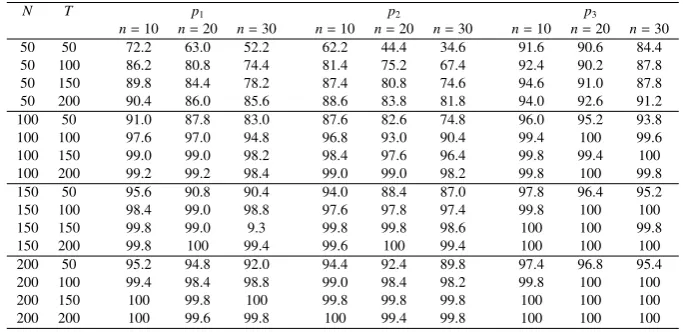
[image:15.595.129.468.454.646.2]Table 3: Probabilities of Correctly Identifying IOFs
N T p1 p2 p3
n=10 n=20 n=30 n=10 n=20 n=30 n=10 n=20 n=30
50 50 72.2 63.0 52.2 62.2 44.4 34.6 91.6 90.6 84.4
50 100 86.2 80.8 74.4 81.4 75.2 67.4 92.4 90.2 87.8
50 150 89.8 84.4 78.2 87.4 80.8 74.6 94.6 91.0 87.8
50 200 90.4 86.0 85.6 88.6 83.8 81.8 94.0 92.6 91.2
100 50 91.0 87.8 83.0 87.6 82.6 74.8 96.0 95.2 93.8
100 100 97.6 97.0 94.8 96.8 93.0 90.4 99.4 100 99.6
100 150 99.0 99.0 98.2 98.4 97.6 96.4 99.8 99.4 100
100 200 99.2 99.2 98.4 99.0 99.0 98.2 99.8 100 99.8
150 50 95.6 90.8 90.4 94.0 88.4 87.0 97.8 96.4 95.2
150 100 98.4 99.0 98.8 97.6 97.8 97.4 99.8 100 100
150 150 99.8 99.0 9.3 99.8 99.8 98.6 100 100 99.8
150 200 99.8 100 99.4 99.6 100 99.4 100 100 100
200 50 95.2 94.8 92.0 94.4 92.4 89.8 97.4 96.8 95.4
200 100 99.4 98.4 98.8 99.0 98.4 98.2 99.8 100 100
200 150 100 99.8 100 99.8 99.8 99.8 100 100 100
200 200 100 99.6 99.8 100 99.4 99.8 100 100 100
DGP:xit=∑2k=1λkifkt+eit, whereft=(f1t,f2t)′is multivariate normal withE(fkt)=0,E(fkt2)=1, andE(f1tf2t)=0.5.
f1t =x1t−x2t, f2t=x3t,eit, andλkiare all i.i.d standard normal variables. The reported numbers are the probabilities
of correctly identifying the IOFs:x1:3,tout of 500 replications forn=10,20,30 and 3 different penalty functionsp1,p2 andp3.
6.2. Indirectly observed factors
Now we generate data sets with 2 latent factors and 3 observed factors, i.e.,r=2 andm=3. The first latent factor is the difference of the first two observed variables: f1t=x1t−x2t, and the
second latent factors is equal to the third observed variables: f2t=x3t. Therefore we can write:
ft=
(
1 −1 0 0 0 1
)
x1:3,t.
The other parts of the models are generated as in Section 6.1. We use the method described in Section 4 to identify the IOFs, withrmax = 4. To reduce the computation cost, we restrict
the search to subsets of the variables that contain the IOFs. As discussed in Section 4, the less variables we consider, the more likely that the IOFs are identified. The results from 500 replications forn=10,20,30 are reported in Table 3, which shows the probabilities of correctly identifying both the number of IOFs (m=3) and the IOFs.
Several conclusions can be drawn. First, our method performs well in most cases, with high probabilities (more than 80%) of correct identification. Secondly, p1(N,T) performs best
among the three penalty functions we consider. Thirdly, the probabilities of correct identification decrease as we increase the number of variables (n) that include the IOFs, but the reductions are not sharp. For most cases, they are less than 2% when we include 10 extra variables in the searching process.
Next we compare our test statistics proposed in Section 5 to those of Bai and Ng (2006). The discussions in Section 4 implies that for the DGPs considered here, the tests of Bai and Ng (2006) will identifyx3t as an observed factor but will reject the null hypothesis forx1tandx2t,
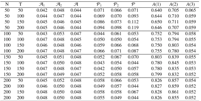
while our test should identify all of the three observed factors. The simulation results from 1000 replications are reported in Table 4.
Table 4: Test with IOFs
N T A1 A2 A P1 P2 P A(1) A(2) A(3)
50 50 0.042 0.048 0.044 0.071 0.066 0.071 0.640 0.705 0.065
50 100 0.044 0.047 0.044 0.069 0.070 0.093 0.644 0.710 0.059
50 150 0.045 0.046 0.045 0.086 0.073 0.112 0.650 0.711 0.059
50 200 0.045 0.046 0.044 0.094 0.098 0.119 0.646 0.707 0.059
100 50 0.043 0.053 0.047 0.044 0.061 0.053 0.752 0.794 0.058
100 100 0.047 0.048 0.045 0.050 0.050 0.054 0.753 0.794 0.055
100 150 0.046 0.048 0.046 0.059 0.066 0.068 0.750 0.803 0.054
100 200 0.047 0.048 0.047 0.066 0.071 0.087 0.755 0.780 0.054
150 50 0.045 0.051 0.048 0.052 0.067 0.070 0.803 0.839 0.055
150 100 0.047 0.050 0.048 0.043 0.054 0.044 0.780 0.845 0.053
150 150 0.047 0.048 0.047 0.042 0.050 0.057 0.780 0.835 0.053
150 200 0.047 0.049 0.047 0.052 0.058 0.058 0.799 0.832 0.052
200 50 0.045 0.052 0.048 0.058 0.066 0.053 0.826 0.857 0.054
200 100 0.046 0.050 0.048 0.049 0.057 0.044 0.827 0.859 0.052
200 150 0.048 0.050 0.048 0.058 0.058 0.067 0.828 0.861 0.052
200 200 0.048 0.050 0.048 0.055 0.049 0.044 0.826 0.855 0.052
Note: The DGPs are the same as in Table 3. In Columns 3 to 5 are the averaged values ofAkfrom 1000 replications. In Columns 6 to 8 are the empirical sizes of the testsPkcorresponding to the 5% critical value. In Columns 9 to 11 are the averaged values of theA(j) tests of Bai and Ng (2006).
It can be seen that our tests (columns 3 to 8) still perform good for the all the sample sizes considered, although ourPktests are oversized for small sample sizes. However, theA(j) tests
of Bai and Ng (2006) (columns 9 to 12), based on the regressions of IOFs on the estimated factors, fail to converge to 5% for the first two observed factors because they are not directly observed (x1t −x2t = f1t). Their tests can only identify x3t as an observed factor because it
directly approximates f2t. Hence, these simulation results confirm the superiority of our test in
the case of IOFs.
7. Applications
7.1. Data sets
In this part, we use our method to identify the underlying factors that determine the excess returns of portfolios. It is well known that the Fama-French (FF henceforce) 3 factors, including Market excess return (Market), Small Minus Big (SMB) and High Minus Low (HML), are good approximates of the unobservable risk factors, in the sense that they can explain well the vari-ances of the returns. The purpose of the application is to see that, given that the FF 3 factors are the observed counterpart of the underlying risk factors, and that the estimated factors using PC are consistent for the underlying factors, if our method can successfully identify these 3 factors among a panel of other observed variables. One the other hand, if our method fails to identify the FF 3 factors, we should question the consistency of the estimated factors, or the validity of the FF 3 factors as approximations of the underlying risk factors.
We use two data sets in our empirical study. The first data set consists of the monthly re-turns of 100 portfolios formed on Size and Book-to-Market, which can be downloaded from the webpage of Kenneth French together with the FF 3 factors. The second data set consists of 151
monthly macro series taken from Stock and Watson (2002b), including variables such as indus-trial production, employment, prices, interest rates, and exchange rates. The macro variables are transformed to achieve stationarity, and the transformation methods for each variable can be found in Stock and Watson (2002b). Both data sets range from 1960 to 1997 (T=444).
We first estimate the factors from the panel of portfolio returns, and then identify the observed factors from the macro data set and FF 3 factors. Beside the FF 3 factors, it is widely believed that asset returns are also commonly affected by some macro fundamentals. The use of the macro data set allows us to find the possible connections between macro variables and financial markets.
7.2. The number of factors
Before estimating the factors, an important question is how many factors are there. We use two different methods to determine the number of factors for both data sets. The first one is the information criteria (IC) method of Bai and Ng (2002), which penalizes extra factors in a proper way such that the penalty functions help to choose the right number of factors. The second one is Onatski (2010), which is based on the fact that in a factor model withrfactors, only the largest reigenvalues of the covariance matrix explode as the number of variables go to infinity, while the remaining eigenvalues are bounded. The method of Bai and Ng (2002) is usually criticized for overestimating the number of factors, the method of Onatski (2010) is shown to have better finite sample performance when there are non-trivial cross sectional correlations between the idiosyncratic errors.
[image:18.595.136.474.487.564.2]The estimation results for the number of factors are reported in Table 1. It can be seen that for the panel of portfolio returns, 3 to 5 factors are found using different ICs of Bai and Ng (2002), while Onatskis method identifies 3 factors. For the macro data set, the estimated numbers using ICs are all 10, much larger compared to the number (3) found by Onatskis method.
Table 5: The estimated number of factors using the information criteria of Bai and Ng (2002) and the method of Onatski
(2010), withrmak=10.
Samples PC1 PC2 PC3 IC1 IC2 IC3 Onatski T N
Portfolios 1960-1996 5 4 5 3 3 3 3 444 94
1960-1980 5 4 6 3 3 4 4 240 94
1980-1996 5 4 7 4 3 5 3 204 94
Macro 1960-1996 10 10 10 10 10 10 3 444 153
Variables 1960-1980 10 9 10 10 8 10 4 240 153
1980-1996 10 10 10 10 10 10 3 204 153
We then split the sample by 1980 (for reasons discussed below) and estimate the number factors for each subsamples. The results from Onatski (2009) is the same for both data sets: 4 factors for samples from 1960 to 1980 and 3 factors from 1980 to 1997. The results from Bai and Ng (2002) are less consistent: for the financial data set, the estimated numbers range from 3 to 7 for the two subsamples, and the estimated numbers from subsamples are usually larger than those from the full sample. For the macro data set, the selected numbers of factors using ICs are almost all 10 for each subsamples.
As discussed in Chen Dolado and Gonzalo (2011), the differences in the numbers of factors between subsamples and full sample usually imply structural breaks in the factor model, e.g., the
breaks in the factor loadings or the change of factor numbers. However, the number of factors in the full sample should be no less than the number of factors in the subsamples, if the number of factors are correctly estimated. Therefore, the differences of the estimated factors between subsamples and full sample are more likely due to the estimation errors of the two methods in finite samples. Finally, the results in Table 1 strongly favors the specification of 3 factors for both data sets in the full sample.
7.3. Testing for structural instability
Structural instabilities are common features of financial and macro data sets, see Stock and Watson (2003) for examples. There are enough reasons to expect that the factor models con-sidered here are subject to some sort of structural instabilities. Breitung and Eickmeier (2011) is the first paper that proposes formal test statistics to test the null hypothesis of constant factor loadings in large dimensional factor models, but their test is shown to suffer from several short-comings by Chen, Dolado and Gonzalo (2011), who propose a new test procedure for the same null hypothesis, which is shown to have power only against big breaks in the factor loadings. It is also argued that the small breaks, which are of order 1/√NT, will not affect the estimation and inference of factor models based on PC methods. A similar test is also proposed by Han and Inoue (2011) independently.
We apply the test of Chen, Dolado and Gonzalo (2011) to both data sets. Their test can be easily implement in two steps. In the first step, the number of factors is chosen or estimated (one can apply the test with different chosen number of factors as we will do here), and the factors are estimated using PC. In the second step, the first estimated factors are regressed on the remaining ones, and a Sup type test of Andrews (1993) is used to test the constancy of the coefficients in this regression. If the null is rejected in the second step, we can conclude that there are big structural breaks in the factor loadings; otherwise there are only mild instabilities that can be safely ignored.
The results with the Sup Wald tests are reported in figures 1 and 2. The chosen numbers of factors range from 3 to 6, consistent with previous findings. For the financial data set, the trimming [0.3,0.7] is used, while for the macro data set, we use [0.05,0.95]. The red dotted lines are critical values (5% for the financial data and 1% for the macro data) of the Sup type test tabulated by Andrews (1993), and the black dotted lines are the critical values of theχ2
r−1(for a
known breaking date, the Wald test converges toχ2 r−1).
The results for the portfolio returns data indicate the existence of a break around 1980, for all the numbers of factors we consider. For the macro data set, the Wald tests strongly reject the null of no structural breaks around 1966 and 1973, implying that there may be multiple breaks during this period. However, the Wald tests for the macro data set can not reject the null at 1% significant level after 1980, even when the tests are compared to the critical values of theχ2 distributions.
It should be noted that the tests of Chen Dolado and Gonzalo (2011) and Han and Inoue (2011) are based on the relationships between estimated factors. Therefore, these tests also have powers against the breaks in the dynamics of the true factors, which can not be differentiated from breaks in the factor loadings from the tests. However, as pointed out by Chen Dolado and Gonzalo (2011), the breaks in the factor loadings and in the factors can be differentiated by comparing the estimated number of factors in the subsamples and the full sample. If the breaks happen in the factors, the estimated number of factors should be the same before and after the break; if the breaks happen in the factor loadings, the estimated number of factors using
the full sample will usually be larger than that using subsamples. This observation, combined with the results of estimated numbers of factors from previous subsection, provides evidences for the presence of breaks in the factor dynamics rather than the factor loadings. To check the consistency of our results, we apply our method in the following subsection to the full sample and the two subsamples. One should keep in mind that for the macro data, the second subsample (post 1980) is more stable according to our testing results.
0 4 8 12 16 20
66 68 70 72 74 76 78 80 82 84 86 88 90
WALD3
0 4 8 12 16 20
66 68 70 72 74 76 78 80 82 84 86 88 90
WALD4
0 4 8 12 16 20 24
66 68 70 72 74 76 78 80 82 84 86 88 90
WALD5
0 4 8 12 16 20 24
66 68 70 72 74 76 78 80 82 84 86 88 90
[image:20.595.117.478.240.448.2]WALD6
Figure 1: Wald tests for the returns of portfolios, with trimming [0.3,0.7]. Red dotted lines: 5% critical values for the Sup type tests. Black dotted lines: 5% critical values forχ2distributions.
0 4 8 12 16 20 24
62 64 66 68 70 72 74 76 78 80 82 84 86 88 90 92 94
WALD3
0 4 8 12 16 20 24 28 32
62 64 66 68 70 72 74 76 78 80 82 84 86 88 90 92 94
WALD4
0 5 10 15 20 25 30 35
62 64 66 68 70 72 74 76 78 80 82 84 86 88 90 92 94
WALD5
0 5 10 15 20 25 30 35 40
62 64 66 68 70 72 74 76 78 80 82 84 86 88 90 92 94
[image:21.595.121.477.151.361.2]WALD6
Figure 2: Wald tests for the macro variables, with trimming [0.05,0.95]. Red dotted lines: 1% critical values for the Sup type tests. Black dotted lines: 1% critical values forχ2distributions.
7.4. Empirical results
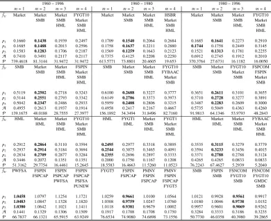
In this subsection, we apply our identification method to find the observed factors in the portfolio returns. We first estimate the factors from the panel of returns, and then form a list of 50 candidates for the observed factors from the panel of macro variables and FF 3 factors, based on their correlations with the estimated factors and their economic meanings. As discussed in Section 4, by creating such a list of candidates, we can significantly reduce the computation cost to an affordable level. The full list of these 50 candidates including their short names, full names and transformation codes are given in the appendix. Besides the FF 3 factors, these 50 candidates include the usual macro variables such as industry production, various interest rates, monetary measures, inflations and consumptions, which have often been considered as the main economic factors that affect the financial market in previous studies.
Finally, we identify the observed factors with each of the estimated factors, starting with the first one, and apply our two type of test statistics to each set of identified observed factors. The results are reported in Table 6.


![Figure 1: Wald tests for the returns of portfolios, with trimming [0.3, 0.7]. Red dotted lines: 5% critical values for theSup type tests](https://thumb-us.123doks.com/thumbv2/123dok_us/7781555.721704/20.595.117.478.240.448/figure-returns-portfolios-trimming-dotted-critical-values-thesup.webp)
![Figure 2: Wald tests for the macro variables, with trimming [0.05, 0.95]. Red dotted lines: 1% critical values for the Suptype tests](https://thumb-us.123doks.com/thumbv2/123dok_us/7781555.721704/21.595.121.477.151.361/figure-wald-variables-trimming-dotted-critical-values-suptype.webp)