Residential Community Open Up Strategy Based on Prim’s Algorithm and Neural Network Algorithm

ISSN Online: 2327-4379 ISSN Print: 2327-4352

Residential Community Open-Up Strategy

Based on Prim’s Algorithm and Neural Network

Algorithm

Ximing Lv

, Ang Li

, Shunkai Zhang

, Jianbao Li

1_{School of Mathematical Sciences, Inner Mongolia University, Hohhot, China}

2_{School of Statistics and Mathematics, Inner Mongolia University of Finance and Economics, Hohhot, China} 3_{School of Finance, Inner Mongolia University of Finance and Economics, Hohhot, China}

Abstract

“Open community” has aroused widespread concern and research. This paper focuses on the system analysis research of the problem that based on statistics including the regression equation fitting function and mathematical theory, combined with the actual effect of camera measurement method, Prim’s algo-rithm and neural network to “Open community” and the applicable condi-tions. Research results show that with the increasing number of roads within the district, the benefit time gradually increased, but each type of district ca-pacity is different.

Keywords

Open Community, Regression Analysis, Prim’s Algorithm, Graph Theory, Neural Net-Work Algorithm

1. Introduction

Capillaries are reticular throughout the body, connecting arteries and veins. If the capillary is clogged, it will affect the blood flow and material exchange be-tween arteries and veins. For urban traffic, “capillaries” are small roads that people are not interested in. If the “capillaries” blocked, then the “artery” and “vein” are no longer efficient [1]. How to solve the problem of traffic congestion by reasonable “open community” to improve the density of the road network is the focus of our study.

In order to study this huge problem, we decided to establish a mathematical model, and then empirical analysis. This requires us to establish a suitable index system, to evaluate the “open community” to control the role of road congestion. How to cite this paper: Lv, X.M., Li, A.,

Zhang, S.K. and Li, J.B. (2017) Residential Community Open-Up Strategy Based on Prim’s Algorithm and Neural Network Algorithm. Journal of Applied Mathematics and Physics, 5, 551-567.

https://doi.org/10.4236/jamp.2017.52047

Received: January 5, 2017 Accepted: February 25, 2017 Published: February 28, 2017

Copyright © 2017 by authors and Scientific Research Publishing Inc. This work is licensed under the Creative Commons Attribution International License (CC BY 4.0).

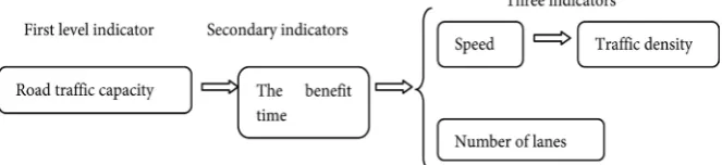
After analysis, we established the following index evaluation system (Figure 1). Road capacity, we can use a certain vehicle through a certain area of the minimum time to measure. The term “the benefit time” is defined as the time difference between a roadway around a residential area that permits traffic and does not allow traffic. The “the benefit time” is determined by the number of lanes and the speed, and the speed is related to the traffic density

2. Data Acquisition and Analysis

2.1. Regional Analysis and Selection

As of September 11, 2016, there were 23 provinces, 4 municipalities, 2 special administrative regions and 5 autonomous regions in China. A total of 660 one, two, three-tier cities, each city car capacity and community structure is different, in order to study the problem in a better environment, select a suitable city is essential [2].

2.1.1. The Selection of Hohhot Region Region selection reason:

1) Motor vehicle ownership is more appropriate, the majority of private cars, Hohhot, China can represent most of the city level, and there is great room for optimization.

2) This city is located in the plateau area. Roads are mostly straight; car con-gestion is almost free from geographical factors.

3) Residential area characterized as “Large mixed, small settlements”, forming a number of residential circle, conducive to the investigation and research.

Based on the above reasons, the selected research city is Hohhot, and the se-lected community is the representative district in this city.

2.1.2. The Selection of Residential Areas

According to the data obtained from the traffic management department of Hohhot, as shown in the blue area for most of the private car owner residential area, the figures (Figure 2) shown are the percentage of private car ownership in the area. In our data, we selected the smallest percentage (red five-pointed star “★_{” mark) area and representative area, as our research area and field} observa-tion area. Traffic flow around it can be approximated according to the following formula:

Traffic flow around the residential area = total traffic volume × The percen-tage.

Figure 2. The map of Hohhot.

Figure 3. “Double hump”.

2.2. Acquisition of Traffic Flow Data

2.2.1. The Average Hourly Traffic Data Acquisition

Through the “2011-2013 focus on environmental protection in key urban road traffic noise monitoring situation (2014)”, we found that the average hourly traf-fic volume in Hohhot was 2231 Vehicle/hour [3].

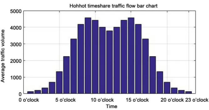
2.2.2. The Trend of the Daily Traffic Volume in Hohhot

Through the study of many authoritative data, we find that the trend of traffic flow in many cities is “double hump [4]” (Figure 3).

Figure 4. Hohhot timeshare flow bar chart.

2

2

3 2

4

y 3 0.5 e 0.1 1000

4

x

x −_ − _ +

_{  } 

 

= _ − _ + _× + ×

_  _ 

 

(1)

In the follow-up analysis, the total traffic volume of the whole city in different time periods will be calculated by this function.

3. Preliminary Results

Through the analysis of the problem, we choose an algorithm in graph theory- Prim’s algorithm [5] [6][7] to resolve this issue. It finds a subset of the edges that form a tree that includes every vertex, where the total weight of all the edges in the tree is minimized. The algorithm operates by building this tree one vertex at a time, from an arbitrary starting vertex, at each step adding the cheapest possible connection from the tree to another vertex. We believe that Prim’s algo-rithm can be a good solution to this problem.

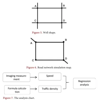
In general, area around the crossroads can be formed well shape(Figure 5). Assume the gate is at points A and D, so departure from A1 and A2 or D1 and D2 the departure traffic is the same. So this situation can be simplified into the following road network simulation map (Figure 6).

3.1.1. Traffic Velocity-Density Relation Model

In order to obtain the necessary data, we use the Traffic Engineering photo-grammetry [8][9][10]. We were erected VCR in Wulanchabu East Road and the pedestrian bridge at University Road. Finally, select a number of private cars in the video, calculate the speed. Assuming constant speed, select one of the repre-sentative speed as the fitting data points in the speed value, in this selection, we assume that the vehicle travels at a constant speed and then uses the representa-tive velocity as the velocity value in the fitted data points, Through the “double hump” function and the surrounding area traffic flow calculation formula, cal-culate the density of different time periods. A total of 24 groups were selected (Figure 7).

Figure 5. Well shape.

Figure 6. Road network simulation map.

Figure 7. The analysis chart.

analysis [11] [12] [13] of the data to quantify the relationship between density and speed.

In order to quantitatively express the relationship between density and veloci-ty, we then carry out different degrees of regression analysis in order to find the function expression between the two.

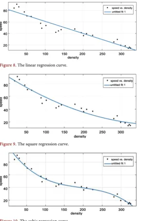
3.1.2. Linear Regression Models

Its linear regression model is shown in Figure 8. 1) Square regression equation

Its square regression model is shown Figure 9. 2) Cubic regression equation

Its cubic regression model is shown in Figure 10. 3) Neural Network Optimal Regression

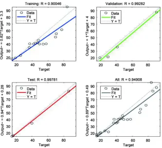
We use MATLAB software for neural network Levenberg-Marquardt [14] [15][16] operation. Set Training 70%, Validation 15%, Text 15%, to obtain the optimal regression curve (Figure 11).

Remnant analysis of neural network and raining, Validation, Text of the cor-relation coefficient are shown in Figure 12 and Figure 13.

Figure 8. The linear regression curve.

Figure 9. The square regression curve.

Figure 10. The cubic regression curve.

Figure 12. Residual analysis of neural network.

Figure 13. Correlation coefficient analysis.

3.1.3. Put Forward the Mathematical Model

According to the Prim’s algorithm and permutation and combination method, we simulate the driver’s route selection method:

1) In the node a wait, in front of the fork in the road 1, 2, ..., after selection into step 2.

to reach the next node, go to step 3.

3) The node is the end of the loop term to stop, if not the end, continue with step 1 cycle.

In the steady state, with the formula for calculating the profit time to get this set of formulas:

(

)

(

)

(

)

(

)

i i i i i i

i i i

T T T T T T T i

∆ =

∑

∑

∑

In which, 1

i

T is the commuting time required before opening section Yi, 2

i

T is the commuting time required after opening section Yi, 3

i

T is the length of the before opening section Yi/the speed of the Vehicle on the road before opening section Yi, 4

i

T is the length of the after opening section Yi/the speed of the ve-hicle on the road after opening section Yi, 5

i

T is the length of the before open-ing section Yi/the traffic density of the before openopen-ing section Yi, 6

i

T is the length of the after opening section Yi/the traffic density of the after opening sec-tion Yi.

3.2. Simple Model Simulation

By simulating the simplest cell structure, we can obtain the following road net-work simulation map (Figure 14).

Let AB segment be n1 lane, BD segment be n2 lane, CD is n3 lane, AC segment is n4 lane.

According to the driver routing method, we can assume that in the case of stability, AE and AC road traffic density is the same. Let this traffic density be ρ_{, And traffic flow density caused by traffic flow in other directions is denoted} by ρn, ρe, ρs, ρw. After opening the cell, the density of each section is

The ratio of traffic density between AE and AC links is 1:1

,

AE=ρ AC=ρ (3) When the vehicle arrives at point E, the traffic density of EF and EB sections is equal. The ratio of traffic density between EB and AE is 1: (1 + n_1):

1 2

1 1

1 1

EB EF

n n

ρ× ρ×

= =

+ ， + (4)

When the vehicle arrives at point B, the traffic density of EB and BD is n1:n2:

(

)

n BD

n n

ρ

+ × (5)

When the vehicle arrives at the point F, the traffic density of the FD section comes from the traffic density of the EF section and the CF section:

4 1 3 1 n n FD n ρ ρ× +

+

=

When the vehicle arrives at point C, the ratio of the traffic flow density of CF

road segment to the traffic flow density of AC link is n3:n4:

4 3 n CF n ρ×

=

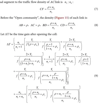
Before the “Open community”, the density (Figure 15) of each link is:

1 4

2 3

n n

AB AC BD CD

n n

ρ ρ

ρ ρ × ×

= ， = ， = ， = ₍₈₎

Let ΔT be the time gain after opening the cell:

(

)

(

)

1 1 2

1

1 1

1

1 2

2 2 2

1 1

1

1 2 2 1

1 1 4 4 1 3 3 2 1 1 1

2 2 2

1 1 1 1 1 1 n n e e e s s

Y Y Y

n f T n f f n n n

Y Y Y

n n

f n f f

n n n n

Y Y n _n f n f n n

ρ ρ ρ _ρ ρ _ρ

ρ _ρ ρ _ρ ρ

ρ ρ _{ρ ρ}

ρ   _{− +} ×   _{+    } ∆ = ₊ ×_ × ₊ × ₊      _{  +   }   ×   × × − _{ } −  × ₊ _+ ×_  × ₊   ×  +        _{+ ×      + }    + −  ×   _{× +}  +    ₊   _ +  1 1 4 4 4 1

1 4 3

3 1 s s Y Y

n n _n

f

n f

n n n

n ρ ρ _{ρ ρ}

ρ          ₋   _{ ×   }  + +  + × _ + _{  + } +  _{   + }    _{ }   (9)

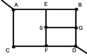
3.2.2. T-Shaped Road District

By modeling a slightly more complex cell structure, we can obtain the following plot road network simulation.

Let AB segment be n1 lane, BD segment be n2 lane, CD is n3 lane, AC segment is n4 lane (Figure 16).

The ratio of traffic density between AE and AC links is 1:1

Figure 16. T-shaped road district.

,

AE=ρ AC=ρ (10) When the vehicle arrives at point E, the traffic density of EB and EO sections is equal. The ratio of traffic density between EB and AE is 1: 1

(

)

1 1 1 , 1 1 EB EO n n

ρ× ρ

= =

+ + (11)

When the vehicle arrives at point B, the traffic density of EB and BD is n1:n2:

(

)

n BG n n

ρ

+ ×

The traffic density of the CF link is determined by the AC link:

4 3 n CF n ρ×

= (13)

When the vehicle arrives at point O, the traffic density of EO is divided into

OG and OF:

1 1

1 1

,

2 2 2 2

OG FO

n n

ρ ρ

× ×

= =

× + × + (14)

The traffic density of the GD section is gathered by the traffic density of the

OG link and the BG link:

(

)

1

1 2

2

1

1 2 2

n n n GD n ρ ρ  × ×  +  _{+ × +}   

= ₍₁₅₎

FG road traffic flow density from the OF section and the CF section of the traffic flow density from the pool, then:

4 1

3

1 2 n n FD n ρ _ρ  ×  + ×  _×   

= ₍₁₆₎

Before the “Open community”, the density (Figure 15) of each link is:

1 2 4 3 , , , n AB BD n n CD AC n ρ ρ ρ _ρ × = = × = = (17)

(

)

(

)

1 1 1 1 2

1 4 1 1

1 1 2

2 2

1

4

1 2 1

3

1 2 2

1 1 1 1 2 2 1 1 1 1 1 2 2 1

1 2 2

n n e

e

e

n

e

n n Y Y Y

T

n n n n

f f f

n n n

Y Y

n

f n

f

n n n

n

Y Y Y

n f n f n n n ρ

ρ _ρ ρ _{ρ ρ}

ρ _ρ ρ _ρ

ρ

ρ ρ _{ρ ρ}   ×  ∆ = × ×_ − + + +      ×  + + +   ₊   ₊             − − _  × ₊   × _{+ ×}  _       _{+ ×}  _{ ×  }   _{+ }  _   × + − +   + × × × ₊ + × +    

(

)

1 4 1

2

2 2 2

1

1 1 1 2

2

1

1 1

2 2 2

2 1

2 2

1 1

1 2 2 1 2 2

n e f n Y Y f n

n f n

n

Y Y

n

f n

f

n n n

n

Y Y Y

n

f f

n n f n n

n

ρ

ρ ρ _ρ

ρ ρ _{ρ ρ}

ρ ρ ρ ρ

  _{ }  _{ }  _ + _   − − _  ×   × _ + ×  _{× +}   _{×  }    _  _   ×  ₊  _{+  } + × ×_ × ₊ + × + _      − − −    ×   × ×  +  ₊   _{× +}    _{+ × +}          1 1 1 4 4 1

1 4 3

3 1 2 s s Y Y

n n _n

f

n f

n n n

n ρ

ρ _{ρ ρ}

ρ         ₋   _{ ×   × }   + ×  + × _ + _{  } × + +  _{   }     _{ }    (18)

Through the empirical analysis of the study, we come to the following conclu-sions as Table 1.

Next, the evaluation system is used to test the traffic flow of the residential ve-hicles: the traffic volume density and the cell type are regulated under the pre-mise of controlling the number of lanes around the cells.

After selecting the mean (175) and maximum (325) in the series data, we found that the same time, the yield time with the number of lanes in the district continues to lengthen. When only the density changes, the experiment chooses the peak data 325, the single-lane cell and the T-shaped road plot gain time is negative, which reflects the two communities on the morning and evening peak

Table 1. The benefit time of a single lane.

Data Sheet

Traffic density The benefit time of a single lane T-section of the benefits of time

170 1.9222 2.6883

traffic capacity is limited. Community open only play a role in slowing traffic congestion, rather than cure.

4. Further Study

4.1. Actual Cell Simulation

This area is a selected area of the old district and the structure is relatively sim-ple. The main road is a one-way street and the main road network structure marked in the map. The area around the road is a two-way street. Now we make an analysis of a problem about whether the area is conducive to ease the sur-rounding road congestion (Figure 17).

Figure 18. The cross-road map.

Through the analysis of the actual map, we get the following road network simulation (Figure 18).

We set the AB segment for the n1 lane, BD segment for the n2 lane, CD for the n3 lane, AC segment for the n4 lane and 1 Lane inside the cell.

After the opening of the district:

According to the principles of the road drivers, the vehicle at A point into the network. AE and AF sections is the same road density so the AE=ρ and

AF =ρ.

At E point because of the density of the EB segment and the EO section, the density ratio of the two sections is n1:1. Then,

1 1

,

1 1

EB EO

n n

ρ ρ

= =

+ + (19)

At F point because of the density of the FC segment and the FO section, the density ratio of the two sections is n4:1.Then,

4 4

,

1 1

FC FO

n n

ρ ρ

= =

+ + (20)

At O point because the density of the OH section and the OG section is the same, the density ratio of the two sections is 1:1 and the traffic volume is the sum of the EO and FO sections. Then,

The traffic flow density of BH and CG sections is fully inherited in EB seg-ment and FC segment. Then,

1 1 4 1 1 1 4 1

,

2 2

n n n n

OH OG

ρ ρ ρ ρ

   

+ +

 _{+ +}   _{+ +} 

   

= = (21)

HD and GD sections of traffic flow density were inherited with BH sections and OH sections with CG sections and OG sections. Then,

1 4 1 4

4 1

4 1

3 2

1 1 1 1

1 2 1 2

,

n n n n

n n

n n

GD HD

n n

ρ ρ ρ ρ

ρ ρ

     

+ +

  _{+ +}    _{+ +}   _{× +}   _{× +} 

 ₊   ₊ 

   

= = ₍₂₂₎

Before the district is not ope, the density of each section:

1 4

2 3

, , , n n

AB BD CD AC

n n

ρ ρ

ρ × × ρ

= = = = (23)

(

)

(

)

2 1

1 2 4

4

4

4 4

4 1

4

2 4 2

1 2

4

4 1 4

1 1 4 1 1 ₁ 1 1

1 1 1

2 n W i i n n D

f D D n

T n _{f D} n

f D D f D D

n n _n

n n n

D D D

f

f n

n

n n n n n

γ γ γ γ γ γ    _{+ − +}    _{+   +}  _{   }  ∆ =_{ }×_ ×_{ + } × +    × + +     _{  }  _ + _  _{ + × }        ₊    _{    }   − ₊ ×_  ₊   ₊ + ₊ _   _  _  _      + + 

(

)

1 2 2

2 1 2 1 2 2 1 1 4 2 1 1 1 1 1 1 1 1 1 1 2 n i e e i n

f D D n n

f D D

n

D D _D

D

D _{f D} f

f D n f n n n

n D γ λ λ λ γ γ  _{+ −}   _{+   −} ×    _{× +}    _{  }     ₊  _ + _       _{   }  _{ } ×_{ + + }− ₊ × _{ +} + _{+   }       _{  } + __  _ + _{ } + _    _{   } (24)

Through the calculation of the data, we come to the conclusion as Table 2: We carried out the following inspection of the district traffic through the evaluation system:

We control the number of lines around the area and cell types as well as the traffic flow density adjustment. As a result, we find that the gain time synchro-nization increases with the increase of density. However, any cell has its upper limit capacity combined with the actual. So it cannot increase the density of traf-fic flow.

4.1.2. Park Type District

This area is within the selected region of a new park area (Figure 19). Gar-den-style design makes the complex structure of the district. Now, we make an analysis of this problem about more complex. The main road is a one-way street. The main road network structure marked in the map and the area around the road is a two-way street.

We will simplify the interior of this area (Figure 20).

Through the calculation of the data, we come to the conclusion as Table 3. Through the analysis of Park Road District, we found that it is the same as the “cross road”. Through the study of the reasons, we find that the park road net-work structure is almost the same as the “cross road” community after the geo-metric transformation. This proves the universality of the “cross road” commu-nity.

5. Results

The State Council of the People’s Republic of China issued the Opinions on Further Strengthening the Management of Urban Planning and Construction, The issue of community Open community has become the focus of attention.

Table 2. The benefit time of cross section.

Data Sheet

Figure 19. The Park type actual cell.

Figure 20. The Park type map.

Table 3. The benefit time of Park-type sections.

Data Sheet

Traffic density 135 142 170 225 325 Park-type sections of the benefit period 3.2172 3.4178 3.9979 7.2684 26.1015

Some people disagree with the Open community of the community, taking into account their own security problems. After the opening of the community, with the passage of vehicles increased in the area, people’s travel security is not guar-anteed, and into the area of mixed personnel, for people’s property security is also a great danger. Therefore, in the construction should pay attention to the construction of security measures and internal road construction in parallel to address people’s concerns.

we must fully consider the choice of road width factors.

6. Conclusions

Through the establishment of the traffic velocity-density relation model, we can see that the one-way and the T-shaped roads have lower bearing capacity. For the simple structure of the internal road area, it cannot make too much traffic flow through, otherwise it will lead to cell blockage. Therefore, it is necessary to control the traffic volume in the district for traffic management. In the daily traffic peak hours, we must set traffic flow access restrictions to prevent exces-sive traffic flow.

Acknowledgements

This research was carried out with support of National Natural Science Founda-tion of People’s Republic of China (project 71261017 and 71661025).

References

[1] Bressack, M.A., Morton, N.S. and Hortop, J. (1987) Group b Streptococcal Sepsis in the Piglet: Effects of Fluid Therapy on Venous Return, Organ Edema, and Organ Blood Flow. Circulation Research, 61, 659-669.

https://doi.org/10.1161/01.RES.61.5.659

[2] Li, J. and Liu, F. (2013) The Planning and Design of Small and Medium Sized Resi-dential Areas in China: Electronic (31).

[3] National Bureau of Statistics of the People’s Republic of China (2014) 2011-2013 Focus on Environmental Protection in Key Urban Road Traffic Noise Monitoring Situation.

http://www.stats.gov.cn/ztjc/ztsj/hjtjzl/2014/201609/t20160918_1400895.html [4] Giese, A., Stolwijk, N.A. and Bracht, H. (2000) Double-Hump Diffusion Profiles of

Copper and Nickel in Germanium Wafers Yielding Vacancy-Related Information. Applied Physics Letters, 77, 642-644. https://doi.org/10.1063/1.127071

[5] Gower, J.C. and Ross, G.J.S. (1969) Minimum Spanning Trees and Single Linkage Cluster Analysis. Applied Statistics, 18, 54-64. http://www.jstor.org/stable/2346439

https://doi.org/10.2307/2346439

[6] Carvalho, B.M., Gau, C.J., Herman, G.T. and Kong, T.Y. (1999) Algorithms for Fuzzy Segmentation. International Conference on Advances in Pattern Recognition, Plymouth, 23-25 November 1998, 154-163.

http://link.springer.com/chapter/10.1007/978-1-4471-0833-7_16

https://doi.org/10.1007/978-1-4471-0833-7_16

[7] Manen, S., Guillaumin, M. and Gool, L.V. (2013) Prime Object Proposals with Randomized Prim’s Algorithm. IEEE International Conference on Computer Vi-sion, Sydney, 1-8 December 2013, 2536-2543.

http://www.cv-foundation.org/openaccess/content_iccv_2013/papers/Manen_Prim e_Object_Proposals_2013_ICCV_paper.pdf

https://doi.org/10.1109/iccv.2013.315

[8] Abdel-Aziz, Y.I. (1971) Direct Linear Transformation from Comparator Coordi-nates in Close-Range Photogrammetry. ASP Symposium on Close-Range Photo-grammetry in Illinois, Champaign, 26-29 January 1971, 1-18.

Pho-togrammetry. Wiley, New York.

[10] Abdel-Aziz, Y.I., Karara, H.M. and Hauck, M. (2015) Direct Linear Transformation from Comparator Coordinates into Object Space Coordinates in Close-Range Pho-togrammetry. Photogrammetric Engineering & Remote Sensing, 81, 103-107.

https://doi.org/10.14358/PERS.81.2.103

[11] Glantz, S.A. and Slinker, B.K. (1990) Primer of Applied Regression and Analysis of Variance. Health Professions Division, McGraw-Hill, New York.

[12] Fox, J. (1997) Applied Regression Analysis, Linear Models, and Related Methods. Sage Publications, Inc., Thousand Oaks.

[13] Montgomery, D.C., Peck, E.A. and Vining, G.G. (2015) Introduction to Linear Re-gression Analysis. John Wiley & Sons, Hoboken.

[14] Qiu, C., Zuo, X., Wang, C. and Wu, J. (2010) A BP Neural Network Based Informa-tion Fusion Method for Urban Traffic Speed EstimaInforma-tion. Engineering Sciences, 8, 77-83.

[15] Chan, K.Y., Dillon, T.S., Singh, J. and Chang, E. (2012) Neural-Network-Based Models for Short-Term Traffic Flow Forecasting Using a Hybrid Exponential Smoothing and Levenberg-Marquardt Algorithm. IEEE Transactions on Intelligent Transportation Systems, 13, 644-654.https://doi.org/10.1109/TITS.2011.2174051

[16] Barba, L. (2014) Forecast of Traffic Accidents Based on Components Extraction and an Autoregressive Neural Network with Levenberg-Marquardt. In: Prasath, R., O’Reilly, P. and Kathirvalavakumar, T., Eds., Mining Intelligence and Knowledge Exploration, Springer International Publishing, New York, 82-90.

https://doi.org/10.1007/978-3-319-13817-6_9

Submit or recommend next manuscript to SCIRP and we will provide best service for you:

Accepting pre-submission inquiries through Email, Facebook, LinkedIn, Twitter, etc. A wide selection of journals (inclusive of 9 subjects, more than 200 journals)

Providing 24-hour high-quality service User-friendly online submission system Fair and swift peer-review system

Efficient typesetting and proofreading procedure

Display of the result of downloads and visits, as well as the number of cited articles Maximum dissemination of your research work

Submit your manuscript at: http://papersubmission.scirp.org/