Modeling Systematic Risk and Point in Time Probability of Default under the Vasicek Asymptotic Single Risk Factor Model Framework

(1)

Munich Personal RePEc Archive

Modeling Systematic Risk and

Point-in-Time Probability of Default

under the Vasicek Asymptotic Single

Risk Factor Model Framework

Yang, Bill Huajian

18 March 2014

Online at

https://mpra.ub.uni-muenchen.de/59025/

(2)

MODELING SYSTEMATIC RISK AND POINT-IN-TIME PROBABILITY OF DEFAULT UNDER THE VASICEK ASYMPTOTIC SINGLE RISK FACTOR MODEL FRAMEWORK

(Pre-typeset version)

(Published in Journal of Risk Model Validation, 8(3), 2014)

BILL HUAJIAN YANG Abstract

Systematic risk has been a focus for stress testing and risk capital assessment. Under the Vasicek

asymptotic single risk factor model framework, entity default risk for a risk homogeneous portfolio divides into two parts: systematic and entity specific. While entity specific risk can be modelled by a probit or logistic model using a relatively short period of portfolio historical data, modeling of systematic risk is more challenging. In practice, most default risk models do not fully or dynamically capture systematic risk. In this paper, we propose an approach to modeling systematic and entity specific risks by parts and then aggregating together analytically. Systematic risk is quantified and modelled by a multifactor Vasicek model with a latent residual, a factor accounting for default contagion and feedback effects. The asymptotic maximum likelihood approach for parameter estimation for this model is equivalent to least squares linear regression. Conditional entity PDs for scenario tests and through-the-cycle entity PD all have analytical solutions. For validation, we model the point-in-time entity PD for a commercial portfolio, and stress the portfolio default risk by shocking the systematic risk factors. Rating migration and portfolio loss are assessed.

Keywords: point-in-time PD, through-the-cycle PD, Vasicek model,systematic risk,entity specific risk, stress testing,rating migration, scenario loss

1. Introduction

Let n denote the size of a portfolio, and k the number of defaults in one-year horizon. Portfolio default rate in horizon is given byrk/n. Assume that the default count k follows a binomial distribution, given the event probability

p

(

s

)

dictated by a latent factor s in horizon. We call

p

(

s

)

the portfolio level probability of default (PD) given systematic risk s in horizon. The quantity

)

(

s

p

contains all information for systematic risk. We can think of

p

(

s

)

as the asymptotic portfolio default rate, when portfolio size is sufficiently large ([12]).

A risk profile x for an entity consists of a vector of current values for a given list of entity specific risk drivers. Let

p

(

s

,

x

)

denote the entity PD in one-year horizon, given systematic risk s and entity risk profile x; and

E

(

p

(

s

,

x

)

|

x

)

the expected value of

p

(

s

,

x

)

given x. We call

p

(

s

,

x

)

the point-in-time (PIT) entity PD, and

E

(

p

(

s

,

x

)

|

x

)

the through-time-cycle (TTC) entity PD ([8]).

Let



denote the cumulative distribution for a standard normal variable. A random variable y,

,

1

0 

y



is said to follow a Vasicek distribution if 1

(

)

y





is normal ([18, p52]). Under the

Vasicek asymptotic single risk factor (ASRF) model framework ([14], [4, p.4-5], [16], [17], [19], [25]), the PIT entity PD for a risk homogenous portfolio (see section 2.1 for definition), as shown in the next section, splits into two parts:

 1(p(s,x))wz, w~ N(



w,



w2), z ~N(0,



z2)



(1.1)

where w and z are mutual independent, w represents the systematic risk depending on s, and z

represents the entity specific risk depending on entity risk profile x.

_{Bill Huajian Yang,, Ph. D in mathematics, Wholesale Credit Methodologies, Bank of Montreal, Toronto,}

(3)

It can be shown (see Proposition 2.3) that, under model (1.1), the systematic risk w and the TTC entity PD are respectively given by:

w



[



1

(

p

(

s

))]

1 



z2



(1.2)

E

(

p

(

s

,

x

)

|

x

)





[(



w



z

)

/

1 



w2

)]

(1.3)

Thus by (1.1) the PIT entity PD is given by:

p

(

s

,

x

)





(

w



z

),

w



[



1

(

p

(

s

))]

1 



z2



(1.4)

To model the PIT and TTC entity PDs, it suffices to model the systematic risk

p

(

s

)

and the entity specific risk z. Each of these risk components can be modelled separately.

The entity specific risk z in model (1.1) canbe modelled by a probit or logistic model targeting a default indicator over a relatively short period of portfolio historical data. In practice, such a model uses a list of entity specific risk drivers x, and is calibrated over the current portfolio to a specific level of systematic risk

s

0

.

We can thus assume that

p

m

(

x

)

is a model for

p

(

s

0

,

x

)

with

systematic risk

s

0

.

Then entity specific risk is given by:

1( ( )) ( 1( ( )))

x p E

x p

z _m   _m (1.5)

where ( 1( ( )))

x p

E  _m denotes the expected value of 1( ( ))

x p_m



 , estimated by the average of

)) ( (

1 x pm



 over the current portfolio.

In contrast, modeling of systematic risk is more challenging due to the data limitation of portfolio historical default rate time series, and the lack of efficient methodologies in parameter estimation. In practice, most PD models do not fully or dynamically capture systematic risk. Default

contagion and feedback effects ([3], [9], [11], [13]) are thus not captured. We will propose in section 2.2 a multifactor Vasicek model with residual for the systematic risk, using the parameter estimation methodology proposed in [27].

As shown in later sections, advantages of the proposed models include:

(a) Systematic and entity specific risk components each is modelled separately, then aggregated together analytically by (1.4).

(b) Conditional entity PDs for scenario tests and entity TTC PDs all have analytical solutions (Propositions 2.3-2.5).

(c) Feedback and default contagion effects are captured and quantified (Propositions 2.4-2.5). (d) Portfolio scenario loss can be assessed (Section 4).

(4)

2. Dynamic Entity PD Models under the Vasicek ASRF Model Framework 2.1. Point-in-Time and Through-the-Cycle Entity PDs

Under the Vasicek ASRF model framework ([14], [4, p.4-5], [16], [17], [19], [25]), default risk in one-year horizon for i-th entity in a portfolio is driven by a normalized latent variable

r

i at time t

(0t12):adefault occurs in horizon if

r

ifalls below a threshold valuecalled default point

d

i,

and the latent variable

r

i splits as:

where s,



i,and



j are the independent variables at time t, with s the systematic risk, and



ithe

entity specific (idiosyncratic) risk. The quantity



i is called the asset correlation. When a risk

profile

x

ifor the i-th entity is observed at current time

(

t



0 )

, we assume



i





i





i, where

i



depends only on

x

i, and ~ (0, ),

2







_i N

with





being

the same for all entities. Given s

and

x

i, the probability of default in horizon for i-th entity is given by





1

(

p

(

s

,

x

i

))







i

/







(

d

i



s



i

)

/(





1 



i

)



Let

z

i



d

i

/(





1 



i

)





i

/









, and

w

i







s



i

/(





1 



i

)

,

where



denotes the average of

d

i

/(





1 



i

)





i

/





over the portfolio. We call

w

i

the

systematic risk and

z

i

the entity specific risk

for i-th entity

.

The portfolio is said to be risk

homogeneous if

w

i

is the same for all entities (i.e., asset correlation is the same for all

entities),

and

z

i

can be regarded as being sampled independently from the same

distribution

N(0,



z2). Then

we have:

 1(p(s,xi))wzi, w~ N(



w,



w2)



(2.1) Suppressing subscript i,we have:

 1(p(s,x))wz, w~N(



w,



w2), z~N(0,



z2)



(2.2)

The following lemma is important for subsequent discussions, where statement (b) is implied by statement (a). Statement (c) (see Appendix for a proof) implies that the volatility of default risk

,

)

(

)

,

(

s

x

w

z

p







given the systematic risk w, is an increasing function of w when w0, a generally desirable property for model (2.2).

Lemma 2.1. Let s~N(



s,



s2), ~ (0, )

2

e

N





. Assume that s and



are independent. Then

(a) ([22, p47])

E

(



(

s





)

|

s

)





(

s

/

1 



e2

)

(b)

E

(



(



))



1 /

2

1 0 ), 1 , 0 ( ~ , ,

1  



 i i i i i

i s s N

r







(5)

(c) Given s, the variance of



(

s





)

is an increasing function of s for

s



0 .

Corollary 2.2. Under model (2.2), theportfolio level PD, given systematic risk s, is:

p

(

s

)



E

(



(

w



z

)

|

s

)





(

s

/

1 



z2

)

By model (2.2), we have the following proposition (see Appendix for a proof).

Proposition 2.3. Under model (2.2), we have:

(a)

w



[



1

(

p

(

s

))]

1 



z2



,

p

(

s

,

x

)





(

w



z

)

(b)

E

(

p

(

s

,

x

)

|

x

)





[(



w



z

)

/

1 



w2

)]

2.2. Multifactor Vasicek Models for Systematic Risk

In this section we propose approaches to modeling

p

(

s

),

i.e., the portfolio level PD in one-year horizon, given systematic risk s. Restriction to risk homogeneity is not required, and the

discussion extends to a general portfolio. Recall that

p

(

s

)

contains all information for systematic risk.

We propose the following multifactor Vasicek model for

p

(

s

)

:

(

)

(

'

)

,

'

~

(

0 ,

2

)

1 1



N

s

b

u

a

s

p

m

j j j j

j k

j









 

(2.3)

where

u

1

,

u

2

,

...,

u

kmeasure current portfolio credit quality, such as current portfolio default rate,

region, and industry sector; while

s

1

,

s

2

,

...,

s

mare external market or macroeconomic variables in

horizon, i.e.,

s

i



s

i

(

t

)

for a time in future with 0t12 in month. Variables

u

1

,

u

2

,

...,

u

k and

m

s

1

,

2

,

...,

are subjected to a transformation by 1





when necessary. The specification for model (2.3) is for stress testing purpose. When the model is used for forecasting, current values for

s

1

,

s

2

,

...,

s

mare then used. The latent factor

s

'

denotes the model residual, a dynamic

accounting for default contagion and feedback effects, capturing all the remaining effects in horizon not explained by

u

1

,

u

2

,

...,

u

k and

s

1

,

s

2

,

...,

s

m, including the effects after time t and

before the end of the horizon.

Let

S



{(

u

₁i

,

u

₂i

,

...,

u

ki

,

s

₁i

,

s

₂i

,

...,

s

mi

,

r

i

)},

1 

i



N

,

be a given multivariate time series

sample with N observations, where

r

i is the portfolio default rate at time i. Let

p

ibe the

unobservable portfolio PD at time i.Parameter estimation for model (2.3) will follow the

asymptotic maximum likelihood approach proposed in [27]. With this approach, portfolio default rate is equated to portfolio level PD, which in general exaggerates the variance of portfolio level PD, causing a bias to parameter estimates. For this reason, we propose a variance correlation as follows.

Variance correction to portfolio default rates:

(a) Assume a constant size n for the portfolio over time. Let

p

0be the expected value of

portfolio level PD over time. Estimate

p

0by the simple average of sample default rates.

Estimate as

v

(

r

)

the sample variance of all

r

i. Then the variance

v

0of portfolio level PD

(6)

v

0



v

(

r

)



[

p

0

(

1 

p

0

)



v

(

r

)]

/(

n



1 )

(b) Let

r

denote the sample average of all

r

i, and

w

0



v

0

/

v

(

r

)

. Replace

r

iby

rr

i:

rr

i



r



(

r

i



r

)

w

0

Note that p₀(1p₀)v(r)(r₁ r₂ ...rN)/N (r₁2 r₂2 ...rN2)/N 0

unless

0 

i

r

or 1 for all i. We thus have

w

₀



v

₀

/

v

(

r

)



1

and

0 

rr

i



1

unless

r

i



0

or 1 for all i. This correction has the advantage of transforming extreme values of 0 and 1 to other regular values between 0 and 1, which would have been an issue for the asymptotic approach with no variance correction. More importantly, the sample variance of

rr

iis now adjusted to the sample

variance

v

0of portfolio level PD.

Next, to estimate the parameters for model (2.3), we equate

p

i, the portfolio PD at time i, to

rr

i,

and set 1( )

i

i p

z  . It was shown ([27], Theorem 4.2) that the maximum likelihood approach

is equivalent to the least squares linear regression, which minimizes the sum-square of errors:

2 1 1 1

)]

(

[



  





m j ji j ji j k j i N i

s

b

u

a

z

where



,the standard deviation of s’ in model (2.3), is estimated as the standard deviation of the model errors.

To address the serial correlation issue for the time series, we will use the bootstrap technique assuming that the time series of residual

s

'

in (2.3) is stationary

. Below are the steps for parameter estimation for model (2.3) proposed in [27].

Steps for parameter estimation for model (2.3):

(i) Do a variance correction to portfolio default rate as proposed, equate

p

i, the portfolio PD,

to the adjusted default rate

rr

i, and set ( )

1

i

i p

z  .

(ii) Generate B (e.g. B= 200) bootstrap samples each is of the same size as the input sample. For each bootstrap sample, train a model of the form (2.3) using least squares linear regression, and estimate the standard deviation



of the model residual.

(iii) For each parameter, calculate the average of all its bootstrap estimates. Select from all bootstrap models the one with parameters the closest to their parameter averages.

2.3. Conditional PDs

Plugging the multifactor Vasicek model (2.3) into model (1.4), we have:

(

,

)

[

1 (

'

)

]

1 1 2

z

s

b

u

a

x

s

p

m j j j i i k i

z









 



(2.4)

wheres'

and

z

are independent,

s'~ N(0,



2),z~ N(0,



z2).Note that by (1.4) the scalar

2

1 



z must be multiplied to

(

'

)

1 1

s

b

u

a

m j j j i i k i





 

before adding to the entity specific

risk z.

(7)

(a)

p

(

s

1

,

...,

s

m

)

- Portfolio level PD given a scenario of systematic risk factors

s

1

,

s

2

,

...,

s

min horizon and current portfolio conditions

u

1

,

u

2

,

...,

u

k.

(b)

p

(

s

1

(

0 ),

...,

s

m

(

0 ))

-Portfolio level PD given current systematic risk factors

s

1

(

0 ),

...,

s

m

(

0 )

and current portfolio conditions

u

1

,

u

2

,

...,

u

k.

(c)

p

(

s

1

,

...,

s

m

,

x

)

- Entity scenario PD given a scenario of the systematic risk factors

s

1

,

s

2

,

...,

s

min horizon, current portfolio conditions

u

1

,

u

2

,

...,

u

k, and entity current risk

profile x.

Using the notations of model (2.3), we define u and v as:



 







m

j j j j

j k

j

s

b

v

u

a

u

1 1

,

We assume that u and v are normal, and the latent factors' in (2.3) is independent of u and v. Let

)

0 (

v

be the current value of v. Regress the horizon value

v

on its current value

v

(

0 )

over a time series sample by a linear regression to get a model:

v



d





_v

v

(

0 )





v

, where d is the

intercept,



v

the parameter for

v

(

0 )

, and v the residual of the regression model. Let

v





denote the standard deviation of v.

The proposition below calculates the portfolio level conditional PDs (See Appendix for a proof).

Proposition 2.4. Under model (2.3), where

'

~

(

0 ,



2

)

N

s

, we have

(a)

p

(

s

₁

,

...,

s

_m

)



E

(



(

u



v



s

'

)

|

s

₁

,

...,

s

_m

,

u

₁

,

...,

u

_k

)





((

u



v

)

/

1 



2

)

(b)

p

(

s

1

(

0 ),

...,

s

m

(

0 ))



E

(



(

u



v



s

)'

|

s

1

(

0 ),

...,

s

m

(

0 ),

u

1

,

...,

u

k

)

1 /

))

0 (

((









2





2





u

d

v

_v

Since



((

_u



_v

)

/

1 



2

)





(

_u



_v

)

_whenever

₍

_u



_v

₎



₀

_{, Proposition 2.4 (a) implies that}

the latent residual effect s' in model (2.3) contributes to an increase to the portfolio level PD whenever



(

u



v

)



1 /

2

.

The proposition below calculates the scenario entity PD (See Appendix for a proof).

Proposition 2.5. Under model (2.4), where '~ (0, 2), ~ (0, 2)

z

N z N

s



, we have

p

(

s

₁

,

...,

s

m

,

x

)



E

(



(

1 



z2

(

u



v



s

'

)



z

)

|

s

₁

,

...,

s

m

,

u

₁

,

...,

u

k

,

x

)





([

1 



z2

(

u



v

)



z

]

/

1 



2

(

1 



z2

)

(2.5)

3. Stress Testing for Portfolio Default Risk

Stress testing is widely used by financial institutions to assess the vulnerability to exceptional but plausible events. It is a tool complementing the existing internal models for capital allocation ([2], [5], [8], [10], [13], [15], [23]). In practice, stress testing focuses on systematic risk, with shocks from the external market or macroeconomic factors ([7], [13], [24]). With the dynamic model (1.4) and model (2.3), stress testing can be conducted through shocking the systematic risk factors in the model (2.3), then propagate to entity default risk by model (1.4). We focus on scenario tests.

(8)

Scenarios for stress testing can either be historical or hypothetical. Hypothetical scenarios are assumed to capture the interdependence of different risk factors between each other and across time ([13, p.67].

For historical scenario tests, market factors are extracted from historical scenarios; while for hypothetical scenario tests, market factors

s

1

,

s

2

,

...,

s

mare to be generated appropriately. We

propose the following steps for generating hypothetical scenarios:

(a) Assume that

s

1

,

s

2

,

...,

s

mare multivariate normal. Estimate the covariance matrix and

denote it by R. Decompose R by the Cholesky algorithm ([20, pp.51-54]) as:

R



G

T

G

, where

G

Tis the transpose of the matrix G

(c) Generate

w

_i

~

N

(

0 ,

1 )

independently, and deliver a scenario as:

m T

T

m G w w w

s s

s , ,..., ) ( , ,..., )

( 1 2  1 2

3.2. Scenario Tests and Loss Assessments

We propose the following steps for a scenario test:

(a) Model systematic risk by a multifactor Vasicekmodel (2.3), following the steps proposed in section 2.2. This includes estimating the model parameters, and the standard deviation



for the latent effects'.

(b) Model entity specific risk by a probit or a logistic model

p

_m

(

x

),

using a list of entity specific risk sensitive drivers x, calibrate the model

p

_m

(

x

)

over the current portfolio, and

set 1( ( )) ( 1( ( )))

x p E

x p

z _m   _m by (1.5).

(c) Given a scenario for the systematic risk factors, calculate entity scenario PD by expression (2.5), and portfolio scenario loss (SL) by:





i j

ij ij i

EAD

LGD

P

Loss

(3.1)

where

P

idenotes the scenario PD for entity i,EADijthe exposure at default for facility j

of entity i, and LGDijthe loss given default for facility j.

4. An Empirical Example – A Dynamic PD Model for a Commercial Portfolio

4.1. Modeling Systematic Default Risk

In this section, we model the portfolio level PD, i.e.,

p

(

s

)

, for a US commercial portfolio, where historical 1-year default rates are available for each quarter between 2006 and 2012.

The delinquency rate for commercial and industry loans (no seasonal adjustment), posted by US Federal Reserve, is available since 1987. This is the macro variable we use for systematic risk modeling. Based on portfolio historical default data, internal portfolio default rate responds to US delinquency rate by a lag of two quarters.

We follow the steps proposed in section 2.2, do a variance correction to the default rates, and bootstrap 200 times. Each time we train a model of the form (4.1) below over the bootstrap sample:

p

(

s

)





(

a



b

₁

u

₁



b

₂

s

₁



cs

"

),

s

"

~

N

(

0 ,

1 )

(4.1)

where

(

1

)

1

r

(9)

1

(

)

1

US

delinquent

rate

in

6 months

s







We then calculate for each of the parameters a,

b

₁

,

b

₂

,

and c, the average its bootstrap estimates, and select from the bootstrap models the one with parameters the closest to their bootstrap averages. This is the final model we will use for systematic risk

p

(

s

)

.

4.2. Modeling Entity Specific Default Risk

For entity specific risk, we train a logistic model over a sample of portfolio historical data, targeting entity default indicator. The sample contains 1161 entities, including all defaults for years 2006-2011, but non-defaults are sampled randomly and proportionally by year for each year in 2006-2012. The model includes six entity specific risk drivers:

1. Debt Service Coverage Ratio 2. Annual Revenue

3. Ratio of Debt to Tangible Net Worth 4. Ratio of Debt to EBITDA

5. Ratio of Cash and Security to Current Liability 6. Years in Business

For assessment of regulatory capital (RC) ([1, pp.59-60]) and expected loss (EL), the model is calibrated at a long-run portfolio PD of 3.1% over the current portfolio (as of September 2012). Denote this model by

p

_m

(

x

),

given entity specific risk profile x. Note that model

p

_m

(

x

)

is not a PIT model yet at the moment.

4.3. Scenario Tests

The portfolio is assumed to be risk homogeneous, e.g., entities have the same systematic risk (i.e. the same asset correlation), and each entity specific risk z can be regarded as being sampled independently from the same distributionN(0,



z2). Then the idiosyncratic risk component z in

(1.4) can be derived by (1.5) using the entity specific risk model

p

_m

(

x

)

developed in section 4.2:

z 1(pm(x)) E( 1(pm(x)))



 _ _





where ( 1( ( )))

x p

E  _m is estimated by the average of 1( ( ))

x p_m



 over current portfolio (as of

September 2012). Estimate the standard deviation



zof z over the portfolio. Then the systematic

risk component w in (1.4) is given by

1 (

1 1 2 1

"

)

2

cs

s

b

u

b

a

w







_z



where

p

(

s

)





(

a



b

₁

u

₁



b

₂

s

₁



cs

"

),

s

"

~

N

(

0 ,

1 ),

is the model developed in section 4.1 for the systematic risk

p

(

s

)

.

Combine w and z together by (1.4). Scenario tests follow the steps (a)-(c) proposed in section 3.2, using the existing portfolio EAD and LGD models for the portfolio. We assume that each of these two models dynamically captures the exposure at default or the loss rate for a facility in the portfolio.

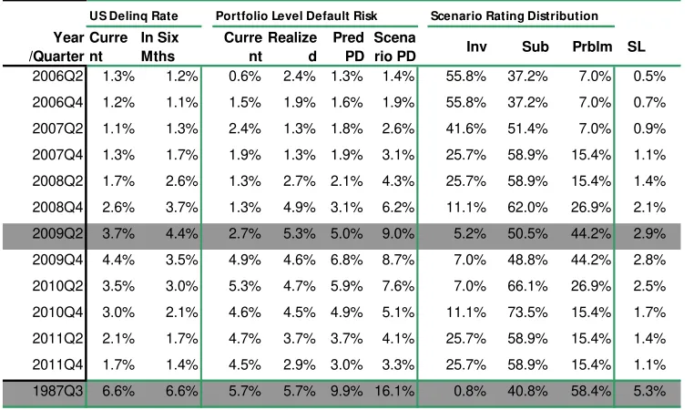
Results are shown in Table 1 below. Entities in the portfolio are grouped into investment (Inv), sub investment (Sub), and problematic (Prblm) grades, based on entity scenario PD given by expression (2.5).

(10)

rate in six months, current portfolio default rate, realized portfolio default rate in one year, predicted portfolio-level PD in one year given by Proposition 2.4(b), and scenario portfolio-level PD given by Proposition 2.4(a). Portfolio scenario loss (SL) is calculated as proposed in Section 3.2 (c), as a percentage of total portfolio exposure (the sum of all facilityEADij in the portfolio).

Recall that the US delinquency rate in six months is the only macro variable used in the model (4.1) for the systematic risk. We are interested in two scenarios as highlighted in Table 1: both assume the current time

(

t



0 )

as of 2nd quarter of 2009.The historical scenario uses the macro variable value of fourth quarter of 2009 (in t 6 months), which is 4.4%, and the hypothetical scenario uses the macro variable value of 3rd quarter of 1987, which is 6.6%.

The results show:

(a) With the hypothetical scenario, most (58.43%) entities migrate to problematic grade (including defaults).

[image:10.612.89.470.319.544.2]

(b) Among all the historical scenarios, portfolio scenario loss (SL) peaks in 2nd quarter of 2010 (the end of one-year horizon), with a loss of 2.9% of the total portfolio exposure; while for the hypothetical scenario, the scenario portfolio loss reaches 5.3% of total portfolio exposure.

Table 1. Scenario assessments for a commercial portfolio

US Delinq Rate Portfolio Level Default Risk Scenario Rating Distribution

Year /Quarter

Curre nt

In Six Mths

Curre nt

Realize d

Pred PD

Scena

rio PD Inv Sub Prblm SL

2006Q2 1.3% 1.2% 0.6% 2.4% 1.3% 1.4% 55.8% 37.2% 7.0% 0.5% 2006Q4 1.2% 1.1% 1.5% 1.9% 1.6% 1.9% 55.8% 37.2% 7.0% 0.7% 2007Q2 1.1% 1.3% 2.4% 1.3% 1.8% 2.6% 41.6% 51.4% 7.0% 0.9% 2007Q4 1.3% 1.7% 1.9% 1.3% 1.9% 3.1% 25.7% 58.9% 15.4% 1.1% 2008Q2 1.7% 2.6% 1.3% 2.7% 2.1% 4.3% 25.7% 58.9% 15.4% 1.4% 2008Q4 2.6% 3.7% 1.3% 4.9% 3.1% 6.2% 11.1% 62.0% 26.9% 2.1% 2009Q2 3.7% 4.4% 2.7% 5.3% 5.0% 9.0% 5.2% 50.5% 44.2% 2.9% 2009Q4 4.4% 3.5% 4.9% 4.6% 6.8% 8.7% 7.0% 48.8% 44.2% 2.8% 2010Q2 3.5% 3.0% 5.3% 4.7% 5.9% 7.6% 7.0% 66.1% 26.9% 2.5% 2010Q4 3.0% 2.1% 4.6% 4.5% 4.9% 5.1% 11.1% 73.5% 15.4% 1.7% 2011Q2 2.1% 1.7% 4.7% 3.7% 3.7% 4.1% 25.7% 58.9% 15.4% 1.4% 2011Q4 1.7% 1.4% 4.5% 2.9% 3.0% 3.3% 25.7% 58.9% 15.4% 1.1% 1987Q3 6.6% 6.6% 5.7% 5.7% 9.9% 16.1% 0.8% 40.8% 58.4% 5.3%

Conclusion. In practice, mostentity PD models do not fully or dynamically capture systematic

risk. The approaches proposed in this paper allow systematic and entity specific risks to be modelled separately and then aggregated together analytically. Systematic risk is quantified and modelled by a multifactor Vasicek model with a latent residual, a factor accounting for default contagion and feedback effects. The asymptotic maximum likelihood approach for parameter estimation for this model is equivalent to least squares linear regression. Conditional entity PDs for scenario tests and TTC entity PD all have analytical solutions. Stress testing can be conducted by shocking the risk factors in the system risk component model.

REFERENCES

(11)

http://www.bis.org/publ/bcbs118.pdf

[2] Basel Committee on Banking Supervision (2009). Principles for Sound Stress Testing Practices and Supervision

[3] Basel Committee on Banking Supervision (2009). The Application of Basel II to Trading Activities and the Treatment of Double default Effects

[4] Basel Committee on Banking Supervision (2005). An Explanatory Note on the Basel II IRB Risk Weight Functions, July 2005.

http://www.bis.org/bcbs/irbriskweight.pdf

[5] Blaschke, W., Jones , M. T., Majnoni, G., and Peria, S. M.(2001). Stress Testing of Financial Systems: An Overview of Issues, Methodologies, and FSAP Experiences, IMF Working Paper, WP/01/88

http://www.imf.org/external/pubs/ft/wp/2001/wp0188.pdf

[6] Breiman, L. (1996). Bagging Predictors. Machine Learning 24: 123-140 http://www.cs.utsa.edu/~bylander/cs6243/breiman96bagging.pdf

[7] Bunn, P. (2005). Stress testing as a tool for assessing systematic risks, Financial Stability Review, 2005:6, pp.116-126

http://www.bankofengland.co.uk/publications/Documents/fsr/2005/fsr18art8.pdf

[8] Carlehed, M., Petrov, A. (2012). A methodology for point-in-time-through-the-cycle probability of default in risk classification systems, Journal of Risk Model Validation, Fall 2012, pp.3-25

[9] Cihak, M. (2007). Introduction to Applied Stress Testing, IMF Working Paper, WP/07/59

[10] Committee on the Global Financial System (2001). A Survey of Stress Tests and Current Practice at Major Financial Institutions

http://www.mirkin.ru/_docs/articles02-055.pdf

[11] Das, S., Duffie, D.,Kapadia, N., Saita, L. (2007) Common Failings: How Corporate Defaults are Correlated. Journal of Finance 62 (1), 93-117

http://www.q-group.org/archives_folder/pdf/Paper-Das.pdf

[12] Demey, P., Jouanin, J., Roget, C, and Roncalli, T. (2004). Maximum likelihood estimate of default correlations, Risk, November 2004

http://thierry-roncalli.com/download/risk-mledc.pdf

[13] Drehmann, M. (2008). Stress tests: Objectives, challenges and modelling choices, Economic Review, 2008:Vol 60 (2), pp. 60-92

http://www.riksbank.se/Upload/Dokument_riksbank/Kat_publicerat

/Artiklar_PV/2008/drehmann2008_2_eng.pdf

[14] Gordy, M. B. (2003). A risk-factor model foundation for ratings-based bank capital rule. Journal of Financial Intermediation12, pp.199-232.

[15] Kupiec P. H. (2000). Stress tests and risk capital, Journal of Risk, Volume 2 (4), pp.27-39

[16] Jacobson, T., Linde, J., Roszbach, K. (2011) Firm Default and Aggregate Fluctuations, Board of Governors of the Federal Reserve System, August 2011

[17] Merton, R. (1974). On the pricing of corporate debt: the risk structure of interest rates. Journal of Finance, Volume 29 (2), 449-470

http://www.jstor.org/discover/10.2307

/2978814?uid=2129&uid=2&uid=70&uid=4&sid=21102236625247

[18] Meyer, C. (2009). Estimation of intra-sector asset correlation. The Journal of Risk Model validation, Volume 3 (3), Fall

http://www.risk.net/digital_assets/5021/jrm_v3n3a3.pdf

[19] Miu, P., Ozdemir, B. (2008). Estimating and validating long-run probability of default with respect to Basel II requirements. The Journal of Risk Model validation, Volume 2/Number 2, 3-41

(12)

[21] Pindyck, R. S., Rubinfeld, D. L. (1998). Econometric Models and Economic Forecasts, 4th Edition, Irwin/McGraw-Hill

[22] Rosen, D., Saunders, D. (2009). Analytical methods for hedging systematic credit risk with linear factor portfolios. Journal of Economic Dynamics & Control, 33 (2009), 37-52 http://www.r2-financial.com/wp-content/uploads/2010/07/LinearFactor.pdf

[23] Segoviano, M. A. and Goodhart, C. (2009). Banking Stability Measures,

IMF working papers 4 (2009).

[24] Tarashev, N., Borio, C., and Tsatsaronis, K. (2010). Attributing systematic risk to individual institutions,” Technical Report Working Papers No 308, BIS, May 2010.

http://www.bis.org/publ/work308.pdf

[25] Vasicek, O. (2002). Loan portfolio value. RISK, December 2002, 160 - 162.

[26] Wolfinger, R. (2008). Fitting Nonlinear Mixed Models with the New NLMIXED Procedure. SAS Institute Inc.

http://www.ats.ucla.edu/stat/sas/library/nlmixedsugi.pdf

[27] Yang, B. H. (2013). Estimating long-run probability of default, asset correlation and portfolio-level probability of default using Vasicek models, Journal of Risk Model Validation, Winter 2013

APPENDIX A

Proof of Lemma 2.1 (c). Given constants a and

b

(



0 )

, it can be shown ([22], Lemma 6, p.48)

that

E a bz c c exp[ (x y 2 xy)/(2 2 )]dxdy

1 2 1 ] )) (

[( 2 2 2

2





_         

 

 

where ca/ 1b2

,





b

2

/

1 

b

2

,

and

z

~

N

(

0 ,

1 ).

By Lemma 2.1 (a), we have

)

1 /

(

)]

(

[

_a

_bz

_a

_b

2

E











. Let



₁denote the derivative of

[(

(

))

2

]

bz

a

E





with respect to

c,

and



₂

the derivative of

2

)])

(

[

(

E



a



bz

with respect to

c

. It suffices to show



₁

>



₂

when

c0

and





0 .

Let



(



)

be the standard normal distribution. Then

,

)

(

)

(

2



c



c





and

we have



_    

 

 c c y cy dy







1 exp[ ( 2 )/(2 2 )]

2

2 2 2 2

2 1



_     



 c c y c dy







1 exp( [ (1 ) ( ) ]/(2 2 ))

2

2 2 2 2 2

2

)

(

)

(

2 ]

)

1 /(

)

1 (

[

)

(

2 )]

2

2 /(

)

(

exp[

1

2 )

(

2

2 2

2

c

dy

c

y

c

















_

















This is because c0and





0 

cc (1



)/(1



) □

Proof of Proposition 2.3. Statement (b) is a corollary of Lemma 2.1 (a). For statement (a), we