Perturbed Planar Restricted Four Body Problem with Repulsive Manev Potential

(1)

ISSN Online: 2333-9721 ISSN Print: 2333-9705

DOI: 10.4236/oalib.1104980 Jun. 6, 2019 1 Open Access Library Journal

Perturbed Planar Restricted Four-Body

Problem with Repulsive Manev Potential

Jagadish Singh

1

, Solomon Okpanachi Omale

2

1_{Department of Mathematics, Faculty of Physical Sciences, Ahmadu Bello University, Zaria, Nigeria}

2_{Engineering and Space Systems Department, National Space Research and Development Agency (NASRDA), Obasanjo Space} Centre, Abuja, Nigeria

Abstract

In this paper, we carried out a numerical study of the planar restricted four-body problem with repulsive Manev potential and perturbations in the Coriolis and centrifugal forces such that the peripherals possess Eulerian con-figuration. We have presented the equations of motion in the rotating frame and investigated the existence and location of the equilibrium points. We have found that there exist six equilibrium points all of which lie along the coordinate axes and shift in positions as the perturbation parameter is varied. We have also examined the linear stability of these equilibrium points and they are found unstable. The dynamical behavior of this system is also inves-tigated using the Lyapunov Characteristic Exponents and the system is found to be chaotic.

Subject Areas

Mathematical Analysis

Keywords

Repulsive-Manev Potential, Coriolis Force, Centrifugal Force, Stability, LCEs, Chaos

1. Introduction

Over the years, Mathematicians and Astronomers have been thrilled by the study of the motion of systems on n-bodies. Sir Isaac Newton pioneered the central-force and two-body problem in his work “Principia” which was first published in [1]. However, the failure of the classical gravitational law to explain the circular moon’s orbit around the earth within the frame of the

in-How to cite this paper: Singh, J. and Omale, S.O. (2019) Perturbed Planar Restricted Four-Body Problem with Repulsive Manev Potential. Open Access Library Journal, 6: e4980.

https://doi.org/10.4236/oalib.1104980

Received: October 11, 2018 Accepted: June 3, 2019 Published: June 6, 2019

This work is licensed under the Creative Commons Attribution International License (CC BY 4.0).

(2)

DOI: 10.4236/oalib.1104980 2 Open Access Library Journal

verse-square force model and other observed phenomena in the solar system dynamics such as the perihelion advances of the inner planets (for instance, mercury), got Newton to study a central-force problem given by a potential of the type 2

A B

r r+ . In Principia’s Book I, Article IX, Proposition XLIV, Theorem XIV, Corollary 2, Newton showed that a central-force problem having this kind of potential leads to precessional elliptic relative orbit. That is, the trajectory of one particle considered with respect to a fixed point moves along an ellipse whose focal axis rotates in the plane of motion. Alexis Clairaut also studied this potential, but finally abandoned it in lieu of the classical poten-tial.

There were other pre- and post-relativistic laws (such as those proposed by Hall and Newcomb) which were able to explain the phenomena of perihelion advances, but unable to justify other issues such as the secular motion of the moon’s perigee. Fortunately, the general relativity theory thrived in expounding well such phenomena in both quantitative and qualitative manner, only with the shortcomings that this powerful theory is not of much help for celestial mechan-ics as all attempts to formulate a meaningful relativistic n-body problem have failed to provide valuable results.

Therefore, the interest is to find a model that can maintain dynamical as-tronomy within the context of classical mechanics, as well as proffering justifica-tions for the observed phenomena as offered by the relativity theory. Such a model meets the theoretical needs of celestial mechanics (by preserving the sim-plicity and advantages of Newtonian mechanics), and can also describe accu-rately the orbits coming close to collisions. By using physical principles, the Bulgarian Physicist George Manev obtained a similar model in the twenties, and proposed an alternative substitute for the relativity theory [2] [3] [4] [5] [6]. In the corresponding central force problem with unit mass for the satellite, Manev’s potential gives A=µ and 22

3 2 B

C

µ

= _{, where}

µ

is the gravitational parameter

of the two-body and C the speed of light. The Manev’s model explains the so-lar-system phenomena with same accuracy as relativity, but without leaving the framework of classical mechanics and it builds a bridge between the classical mechanics and the general relativity. In the recent times, researchers have taken interest in investigating the restricted few-body problem with Manev-type forces [7] [8] [9] [10] [11].

(3)

in-DOI: 10.4236/oalib.1104980 3 Open Access Library Journal

clude various types of effects such as variation of the mass of the primaries, radi-ation pressure force, Poynting-Robertson drag, oblateness of primaries, Coriolis and centrifugal forces, etc. Several researchers such as [12] [13] [14] [15] have considered the effects of small perturbations in the Coriolis and centrifugal forces in the framework of restricted three-body problem.

In this study, our aim is to carry out a numerical investigation of the motion of an infinitesimal mass in the gravitational field of three primaries which are in Eulerian configuration under the effect of small perturbations in the Coriolis and the centrifugal forces together with the bigger primary having a repulsive Manev potential. We studied the equilibrium points, the zero velocity curves, the linear stability and the dynamical behavior of the problem with the restriction that the infinitesimal mass has no influence on the motion of the primary bo-dies.

2. Equations of Motion

We consider the motion of a test particle P of infinitesimal mass m under the gravitational attractions of three bodies P1, P2 and P3 of masses M1, M2 and

3

M respectively, where the gravitational potential of M1 is given by a Manev potential a e₂

r r

 

−_ + _

  with parameter e>0, while the gravitational attraction

due to M2 and M3 is Newtonian

(

−1r

)

. Also, the primaries have Euler configuration such that M2 =M3=µ are located symmetrically with respect to the central body M1, of mass M1 =βµ, which is at the centre of masses of the system (Figure 1). In the inertial frame of reference, the peripherals M2 and M3 move in circular orbits about the central body M1 with angular ve-locity

ω

_{. Now, in a rotating frame Oxyz, we choose the units of the distance,}

mass and time such that the distance between the peripherals is unity and 1

Gµ = _{, where G is the gravitational constant. Let the coordinates of the}

infini-tesimal mass and peripheral masses M1, M2 and M3 be

(

x y,

)

,

( )

0,0 , 1 ,0

2

 

 

  and 1 ,02

₋ 

 

  respectively. As given by [16] and [17], the peripherals

maintain their circular orbit of radius 1 ₂ and angular velocity

ω

_{around the}

central body under the condition that _{ω = ∆}2 _{, where}

(

β,e

)

2 1 4

(

β 16βe

)

∆ = ∆ = + − ₍₁₎

where ∆_{is a positive function, implying the parameter} e>0_{must satisfy the} following sharp bound

0 1 4₁₆

e e β

β +

< = ₍₂₎

(4)

[image:4.595.281.467.75.185.2]

Figure 1. Sketch of the system.

The equations of motion of the infinitesimal mass under small perturbations in the Coriolis and centrifugal forces in the synodic frame can be written as:

2 2

x y

y x

φ

− _{= Ω }



+ _{= Ω }

 

  (3)

where the dots denote time derivatives and the gravitational potential is given as

(

2 2

)

2

1 1 2 3

1 1 1 1

2

x y _e

r r r r

ψ

β

+    

Ω = +   − + + 

∆     (4)

with

(

2 2 2

)

1 1

1

2 ₂

2 2

1

2 ₂

2 3

1 2

r x y

 

= + _

 

_ _ _{ }

=__ − _ +  _ 

 

 

_ _ 



=__ + _ + 

 

 

  

(5)

and

1 , 1,

φ= +ε ε _

1 , 1

ψ = +ε ε′ ′ 

where ε ε ′, are small perturbations given to the Coriolis and the centrifugal forces respectively. The subscripts x and y indicate the partial derivatives of Ω

with respect to x and y respectively. The system (3) possesses the energy integral

2 2 2 ₂

v =x +y = Ω −C (6)

where C is the Jacobi integral constant.

3. Location and Existence of Equilibrium Points

(5)

DOI: 10.4236/oalib.1104980 5 Open Access Library Journal 0

x y x y= = = =

    . It thus follows from Equation (3), that the equilibrium points are solutions of equations

3 4 3 3

1 1 2 3

1 1

1 1 2 2 2 ₀

Δ

x x

e

x x

r r r r

ψ β

  ₋   ₊ 

   

 _ _ _ _{ } _

 

− _ − _ + + =

 _ _ 

 

 

(7)

3 4 3 3

1 1 2 3

1 1 2e 1 1 ₀

y

r r r r

ψ β

    

− − + + =

    

∆  

    

  (8)

we observe that Equations (7) and (8) are independent of φ. This shows that a small perturbation in the Coriolis force has no effect on the positions of equili-brium points.

Theorem (Barrabes et al., 2017); for any β >0 and admissible e, the equi-librium points of the Manev R4BP must lie on the coordinate axes.

Solving Equations (7) and (8) when the centrifugal force is unperturbed (i.e. 1

ψ

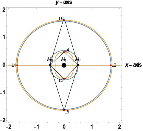
= ), we obtain six equilibrium points lying on the coordinate axes as shown in Figure 2 confirming the theorem (Barrabes et al., 2017) (Table 1).

In Figure 3, we observe that each of the equilibrium points is symmetric to another on the x and y axes respectively and the equilibrium points on the y axis form equilateral triangles with the peripherals M2 and M3.

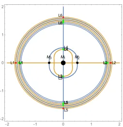
In the perturbed case, we observe that as the centrifugal force perturbation parameter

ψ

increases, the numbers of the equilibrium points does not change but the positions of the equilibrium points with respect to the peripherals change. In Figure 4, we have shown the shifting of equilibrium points.

4. Zero Velocity Surfaces

The energy integral of the problem is given by

2 2

2

C= Ω −x −y (6)

where C is known as Jacobi constant. The curves of zero velocity are defined through 2Ω =C. This relation defines a boundary, called Hill’s surface, which separates regions where motion is allowed or forbidden. Figure 4 shows the zero velocity curves where the problem admits. The value of the Jacobi constant in-creases with increase in the perturbation parameter (Figure 5 and Figure 6). (ψ =1, CL1,2 =9.1949,

ψ

=1.2, CL1,2 =9.72996,

ψ

=1.4, CL1,2=10.2055), ( ψ =1 , CL3,4=13.0987 ,

ψ

=1.2 , CL3,4 =13.1447 ,

ψ

=1.4 ,

3,4 13.1911

CL = ).

5. Linear Stability of the Equilibrium Points

We examine the motion of the infinitesimal body when small displacements are given to the coordinates of the equilibrium point (x0, y0) under consideration.

Let ξ and

η

be these small displacements in the coordinates such that 0

x x= +ξ_and y y= ₀+η_{. Then the variational equations of motion}

(6)

[image:6.595.208.539.91.438.2]

Table 1. Equilibrium points with increase in centrifugal force.

ψ _L_1,2 _L_3,4 _L_5,6

1 (±1.69001, 0) (0, ±0.478827) (0, ±1.63135)

1.1 (±1.63428, 0) (0, ±0.479807) (0, ±1.57227)

1.2 (±1.58505, 0) (0, ±0.480804) (0, ±1.51975)

1.3 (±1.54113, 0) (0, ±0.481817) (0, ±1.47259)

1.4 (±1.50162, 0) (0, ±0.482848) (0, ±1.42986)

[image:6.595.254.494.487.707.2]

Figure 2. Showing the six equilibrium points each lying on the coordinate axes when

β

=10 and e=0.25.

Figure 3. Symmetric equilibrium points.

L1 L2

L3 L4

L5 L6

2 1 0 1 2

x axis

y axis

M1 M2 M3

L1 L2

L3 L4

L5 L6

2 1 0 1 2

x axis

y axis

M1 M2

(7)

Figure 4. Shifts in position of equilibrium points with increase in the centrifugal force.

Figure 5. The zero velocity curves when (ψ =1, CL1,2 =9.1949 , ψ =1.2 ,

1,2 9.72996

CL = , ψ =1.4, CL1,2=10.2055). With the increase in the energy constant

the infinitesimal mass is trapped within the region of each of the primaries.

Figure 6. Zero velocity curves when ( ψ =1 , CL3,4 =13.0987 , ψ =1.2 ,

3,4 13.1447

CL = , ψ =1.4, CL3,4=13.1911). The white region is the region of per-missible motion for the infinitesimal fourth body.

( ) ( )

0 0

2 2

xx xy

ξ η ξ η



− ∅ = Ω + _{Ω }



− ∅ = Ω + _{Ω }

 _

 _ (9)

where the superscript 0 indicates that the values are evaluated at the equilibrium point (x0, y0), the subscripts represent the second partial derivatives and the dots

signify the derivatives with respect to the actual time t. Here the linear terms in

L1 L2

L3 L4

L5 L6

L1 L2

L3 L4

L5 L6

L1 L2

L3 L4

L5 L6

L1 L2

L3 L4

L5 L6

L1 L2

L3 L4

L5 L6

2 1 0 1 2

M1 M2

[image:7.595.247.502.62.326.2]

(8)

DOI: 10.4236/oalib.1104980 8 Open Access Library Journal ξ and

η

_{are only considered.}

Let the trial solutions of Equations (9) be e ,t et

P λ Q λ

ξ = η= ₍₁₀₎

where P Q, are constants and

λ

_{is a parameter. Then the characteristic}

equa-tion of the system (10) can be written as 4 _a 2 _b ₀

λ + λ + = ₍₁₁₎

With

2 0 0

4 xx yy

a=

φ

− Ω − Ω

( )

2

0 0 0

xx yy xy

b= Ω Ω − Ω

(

)

(

)

2

2 2

0

3 5 4 6 5

10 10 10 10 20

2

3 5 3

20 30 30

3 1 2

1 1 3 2 8

3 1 2

1 1

xx

x

x e ex

r r r r r

x

r r r

ψ β  −

Ω = + _{ }− + + − +

∆     + − + −   (12)

2 2 2 2

0

3 5 4 6 5 3 5 3

10 10 10 10 20 20 30 30

1 1 3 2 8 3 1 3 1

yy ψ β _r _ry _re ey_r _ry _r _ry _r

   

Ω = + _ _− + + − _+ − + − _

∆     (13)

0

5 6 5 5

10 10 20 30

1 1

3 3

1 3 8 2 2

xy

x y x y

xy exy

r r r r

β

  ₋   ₊  

   

 _ _ _ _ _ _ 

 

Ω =  − + +

∆  _ _ 

 

 

(14)

(

2 2 2

)

1

10 0 0

1

2 ₂

2

20 0 0

1

2 2

2

30 0 0

1 2

r x y

= + _ _  =__ − _ + _     _ _  =__ + _ + _    

[image:8.595.226.541.150.532.2]

The four roots of the characteristic Equation (11) play an important role in the determination of stability of the equilibrium points. An equilibrium point under consideration will be stable if the Equation (11) has all four purely imagi-nary roots or has four complex roots with each of them having negative real part. This is equivalent to saying that the following system of inequalities must be si-multaneously satisfied (Table 2).

Table 2. Stability of Equilibrium points.

Equilibrium Points λ1,2 λ3,4 Motion

L1,2 (±1.69001, 0) ±0.388944 ±1.17645i unstable

L3,4 (0, ±0.478827) ±2.09503 ±7.2765i unstable

(9)

(

₂ ₀ ₀

)

2

(

₀ ₀

( )

₀ 2

)

4

φ

− Ω − Ωxx yy − Ω Ω − Ω4 xx yy xy >0

(

₄ 2 0 0

)

₀

xx yy

φ − Ω − Ω >

( )

(

₀ ₀ ₀ 2

)

0

xx yy xy

Ω Ω − Ω >

We have computed the characteristic roots of Equation (11) as perturbation parameters φ and

ψ

_{increase and we observe that the equilibrium points L}_i_(i

= 1, 2, 3, 4, 5, 6) are unstable.

6. Dynamic Behaviour of the System

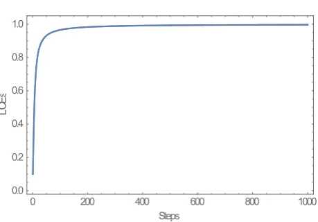
The Lyapunov Characteristic Exponents (LCEs) measure the average rate of convergence or divergence of orbits starting from nearby orbits. It tells whether or not two points in the phase space of a dynamical system that are initially very close will remain close as the motion of the system proceed. It is used as a tool to describe the behaviour of the dynamical systems. It is employed to determine the existence of chaos or regularity of the orbits (for example see [18]). In the appli-cable sense, the exponential divergence of the orbits connotes impossibility to predict the system, so according to [19] any system with at least one positive Lyapunov exponent is chaotic. Therefore, LCEs can be used to analyze the sta-bility of limit sets and to check sensitive dependence on initial conditions, that is, the presence of chaotic attractors (Figure 7).

We have computed numerically the first order LCEs and plotted the graphs (LCEs vs Steps) with the help of Mathematica package developed by Sandri [20]. It is a customary practice to refer to the Maximal Lyapunov Exponent (MLE), because it determines a notion of predictability for a dynamical system. We find that the system is chaotic because the LCEs [0.965343, 0.965343, −0.965343, −0.965343] contain two positive exponents.

7. Discussion and Conclusion

(10)

[image:10.595.259.489.60.220.2]

Figure 7. The Lyapunov Characteristic Exponents of the system.

are unstable. With the aid of Mathematica package, we also computed the LCEs of the system and found that the system is chaotic, because two of its exponents are positive.

Conflicts of Interest

The authors declare no conflicts of interest regarding the publication of this pa-per.

References

[1] Newton, I. (1999) The Principia: Mathematical Principles of Natural Philosophy. University of California Press, ‎Oakland, CA.

[2] Maneff, G. (1924) La gravitation et le principe de l’egalie de l’action et de la reac-tion. Comptes Rendus de l’Académie des Sciences de Paris, 178, 2159-2161. [3] Maneff, G. (1925) Die Gravitation und das Prinzip von Wirkung und

Gegenwir-kung. Zeitschrift für Physik, 31, 786-802. https://doi.org/10.1007/BF02980633

[4] Maneff, G. (1929) Die Masse der Feldenergie und die Gravitation. Astronomische Nachrichten, 236, 401-406. https://doi.org/10.1002/asna.19292362402

[5] Maneff, G. (1930) La gravitation et l’energie au zero. Comptes Rendus de l’Académie des Sciences de Paris, 190, 1374-1377.

[6] Blaga, C. (2015) Prescessing Orbits, Central Forces and Manev Potential. In: Gerd-jikov, V. and Tsetkov, M., Eds., Prof. G. Manev’s Legacy in Contemporary Aspects of Astronomy, Theoretical and Gravitational Physics, Heron Press Ltd., Chicago, IL, 134-139.

[7] Ivanov, R. and Prodanov, E. (2005) Manev Potential and General Relativity. In: Gerdjikov, V. and Tsetkov, M., Eds., Prof. G. Manev’s Legacy in Contemporary As-pects of Astronomy, Theoretical and Gravitational Physics, Heron Press Ltd., Chi-cago, IL, 148-154.

[8] Haranas, I. and Mioc, V. (2009) Manev Potential and Satellite Orbits. Romanian Astronomical Journal, 19, 153-166.

[9] Kirk, S., Haranas, I. and Gkigkitzis, I. (2013) Satellite Motion in a Manev Potential with Drag. Astrophysics and Space Science, 344, 313-320.

https://doi.org/10.1007/s10509-012-1330-0

[10] Blaga, C. (2015) Stability in Sense of Lyapunov of Circular Orbits in Manev

Poten-0 200 400 600 800 1000

0.0 0.2 0.4 0.6 0.8 1.0

Steps

LCE

(11)

DOI: 10.4236/oalib.1104980 11 Open Access Library Journal tial. Romanian Astronomical Journal, 25, 233-240.

[11] Barrabes, E., Cors, J. and Vidal, C. (2017) Spatial Collinear Restricted Four Body Problem with Repulsive Manev Potential. Celestial Mechanics and Dynamical As-tronomy, 129, 153-176. https://doi.org/10.1007/s10569-017-9771-y

[12] Bhatnager, K.P. and Hallan, P.P. (1978) Effect of Perturbations in Coriolis and Cen-trifugal Forces on the Stability of Liberation Points in the Restricted Problem. Ce-lestial mechanics, 18, 105-112. https://doi.org/10.1007/BF01228710

[13] Singh, J. and Vincent, A.E. (2015) Effect of Perturbations in the Coriolis and Cen-trifugal Forces on the Stability of Equilibrium Points in the Restricted Four-Body Problem. Few-Body Systems, 56, 713-723.

https://doi.org/10.1007/s00601-015-1019-3

[14] Abdul Raheem, A. and Singh, J. (2006) Combined Effects of Perturbations, Radiation, and Oblateness on Stability of Equilibrium Points in the Restricted Three-Body Prob-lem. The Astronomical Journal, 131, 1880-1885. https://doi.org/10.1086/499300

[15] Abouelmagad, I.A., Asiri, H.M. and Sharaf, M.A. (2013) The Effect of Oblateness in the Perturbed Restricted Three-Body Problem. Meccanica, 48, 2479-2490.

https://doi.org/10.1007/s11012-013-9762-3

[16] Arribas, M., Elipe, A. and Kalvouridis, T. (2007) Periodic Solutions in the Planar (n+1) Ring Problem with Oblateness. Journal of Guidance, and Dynamics, 30, 1640-1648. https://doi.org/10.2514/1.29524

[17] Fakis, D.G. and Kalvouridis, T.J. (2013) Dynamics of a Small Body under the Action of a Maxwell Ring-Type N-Body System with a Spheroidal Central Body. Celestial Mechanics and Dynamical Astronomy, 116, 229-240.

https://doi.org/10.1007/s10569-013-9484-9

[18] Kumari, R. and Kushvah, B.S. (2013) Equilibrium Points and Zero Velocity Surfaces in the Restricted Four-Body Problem with Solar Wind Drag. Astrophysics and Space Science, 344, 347-359. https://doi.org/10.1007/s10509-012-1340-y

[19] Dubeibe, F.L. and Bermudez-Almanza, L.D. (2013) Optimal Conditions for the Numerical Calculation of the Largest Lyapunov Exponent for Systems of Ordinary Differential Equations. International Journal of Modern Physics C, 25, Article ID: 1450024. https://doi.org/10.1142/S0129183114500247