Parameter Estimations for Generalized RayleighDistribution under Progressively Type I IntervalCensored Data

American Open Journal of Statistics,2011, 1, 46-57

doi:10.4236/ojs.2011.12006 Published Online July 2011 (http://www.SciRP.org/journal/ojs)

Parameter Estimations for Generalized Rayleigh

Distribution under Progressively Type-I Interval

Censored Data

Y. L. Lio1, Din-Geng Chen2, Tzong-Ru Tsai3 1

Department of Mathematical Sciences, University of South Dakota, Vermillion, USA 2

School of Nursing, University of Rochester Medical Center, Rochester, USA 3

Department of Statistics, Tamkang University, Taipei, China

E-mail:[email protected], [email protected], [email protected] Received May 3, 2011; revised May 27, 2011; accepted June 4, 2011

Abstract

In this paper, inference on parameter estimation of the generalized Rayleigh distribution are investigated for progressively type-I interval censored samples. The estimators of distribution parameters via maximum like-lihood, moment method and probability plot are derived, and their performance are compared based on simulation results in terms of the mean squared error and bias. A case application of plasma cell myeloma data is used for illustrating the proposed estimation methods.

Keywords: Maximum Likelihood Estimate, Method of Moments, EM Algorithm, Type-I Interval Censoring

1. Introduction

Burr [1] introduced twelve families of distributions for modeling lifetime data. Among those families, Burr type X and Burr type XII have received the most attention. The Burr type X distribution is also known as the generalized Rayleigh distribution (GRD). The probabi- lity density function (pdf), cumulative distri-bution func- tion (cdf) and hazard function of the two-parameter GRD are defined, respectively, as below:











 2



1  2

2

; , = 2 1 e t e t ,

f t t

 

    _    

(1.1)







 2



; , = 1 e t ,

F t

 

  _ 

(1.2)









 





 

 





2 2

2

1 2

2 1 e e

; , = ,

1 1 e

> 0, > 0, > 0,

t t

t

x h t

t



 

 

   

 



 





  (1.3)

where  is the shape parameter and  is the scale parameter. If  = 1, the GRD reduces to the Rayleigh distribution. The GRD has been studied in many papers such as [2-11]. Johnson et al. [12] provided an excellent review for the GRD up to the year of 1995.

When  1 2, the GRD has a decreasing pdf (1.1) and a bathtub-type hazard function. When  1 2, the pdf (1.1) is a right-skewed unimodal function and the hazard function is an increasing function. The two- parameter GRD has several properties commonly happened in the two-parameter gamma, Weibull and generalized exponential distributions. However, when

1 2

  , the hazard function (1.3) behaves more close to the hazard function of Weibull with shape parameter greater than 1. Similar to the generalized exponential distribution and Weibull distribution, the GRD has a closed form of cdf and is very popular for dealing with censored data. Readers can refer to [5] and [7] for more detailed information about the comparison among these distributions.

Y. L. LIO ET AL. 47

type-II censoring and progressive censoring. The life testing is ended at a pre-scheduled time for the type-I censoring and for the type-II, the life testing is ended whenever the number of lifetimes is reached. Both the type-I and the type-II censoring schemes allow with- drawing the test items only at the end of life testing. However, the progressive censoring schemes allow re- moving test items at some other times before the end of life testing. More information about progressive type-I and type-II censoring schemes and their applications can be found in [13].

Aggarwala [14] introduced the statistical inference procedure for progressively type-I interval censored data from the exponential distribution. Under progressive type-I interval censoring, observations are only known within two consecutively pre-scheduled times and items would be allowed to withdraw at pre-scheduled time points. Ng and Wang [15] studied parameter estimations for Weibull distribution under progressive type-I interval censoring. Chen and Lio [16] inferred the parameters of GED according to progressively type-I interval censored samples. To our best knowledge, there no any research work about the statistical inference for the GRD based on progressively type-I interval censored samples has been published in literatures.

The rest of this article is organized as follows. In Section 2, we introduce the progressive type-I interval censoring scheme into the GRD followed by the theoretical backgrounds and methods for its parameter estimation. A simulation study is conducted in Section 3 to compare the performance of these estimation methods in terms of the mean squared error (MSE) and bias. In Section 4, the application to a real data set is discussed. Some conclusions are given in Section 5.

2. Data, Likelihood and Parameter

Estimations

2.1. Progressively Type-I Interval Censored Data Let items are placed on a life test simultaneously at the initial time 0 and under inspection at m pre-specified times 1 2 , where m is the scheduled time to terminate the experiment. At the time

i, the number, i

n

= 0 t

< < < m

t t  t t

t X , of failures occurred in



ti1,ti



is recorded and i surviving items are randomly removed from the life test, for . At the time m, all surviving items are removed and the life test is terminated. Since the number, i, of surviving items in

R

= 1, 2, ,

i  

Y

1

m t



1



is a random variable and i i at schedule time i, i could be determinated by the pre-specified percentage of the remaining surviving units at the time . For example, given pre-specified percentage values,

and , for withdrawing at

1 2 , respectively, at each inspection time ti where . Therefore, a progressively type-I interval censored sample can be denoted as

,

i t

t

, ,

p 

i

t R Y

R

1 pm1

i

t

= 1

m

p

< < < _m

t t  t R_i =p y_{i i}

, 2, ,

i  m



= 1



X R t_i, _i, _i



, =1, 2, ,



R



i

m

1, 2,,m1



= 0, =

R i

, where sample size

=1 i

i . If i , then the

progressively type-I interval censored sample is a conventional type-I interval censored sample.

= m i

n



X 

2.2. Likelihood Function

Given a progressively type-I interval censored sample,



X R t_i, _i, _i



, = 1, 2,i ,m, of size , from a continuous lifetime distribution with cdf,

n



;



F T  , where  is the parameter vector, the likelihood function can be constructed as follows (see for example, [1]):

 

=1 m

i

L F



t_i,



F t



_i1,



Xi 1





Ri i

F t .

  _     _{ } 

= =

R R 









(2.1)

It can be seen easily that if 1 2 m1 , the likelihood function (2.1) reduces to the corresponding likelihood function for the conventional type-I interval censoring. The maximum likelihood estimate (MLE) for the parameter can be carried out by maximizing the likelihood function of (2.1). Generally, it is often the case without a closed form for the MLE and therefore an iterative numerical search could be used to obtain the MLE from the above likelihood function.

=R _ = 0

2.3. Maximum Likelihood Estimation

Given a progressively type-I interval censored sample from the GRD defined by Equation (1.1) and Equation (1.2), the likelihood function, (2.1), can be specified as follows:

 







 



 





1

2

1 e

.

i i

t t

Ri

 





 2  2

e

e i

Xi

t

 

 

=1

m

i

L  , 1

1 1

 

 _    _

 



 

 

 

 



2

=

(2.2)

Let   . By setting the derivatives of the log likelihood function with respect to  or  to zero, the MLEs of  and  are the solutions to the following likelihood equations



















 



1

2 2

2

2 =1

1 ₂ 1 ₂

2 2

1

=1

e 1 e

1 1 e

1 e e e

=

1 e

t_i t_i m i i

t

i _i

t t t_i t_i

i i i

m

i

R t

X t t



 

 

 

 

 

  



 

   

 

 

2 2

2 2

1

1 e

1 e

i i

t_i t_i

 

 

 _{ }

 



 

 

 





  

and



 









 





 





 





 



2 2 2 =1 2 2 2 2 =1 ₁ 2 2 1 1 2 2 =1 1

1 e 1 e

1 1 e

1 e ln 1 e =

1 e 1 e

1 e ln 1 e .

1 e 1 e

t_i t_i i

m

t

i _i

t_i t_i

m i

t t

i _{i i}

t_i t_i

m

t t

i i i

R ln X                          _{ }  _ _  _{ }  _  _                 







(2.4)

No closed form of the solution can be found to the above equations, and an iterative numerical search can be used to obtain the MLEs. Let ˆMLE and ˆMLE be the solution to the above equations. Then the MLE for  is

MLE MLE

ˆ _{= ˆ}

  . When  is known and  is un- known, then only  needs to be estimated and the MLE is the solution of  to the Equation (2.4) with  replaced by the known 2. When  is known and  is unknown, then on ly  needs to be estimated and the MLE of  is the positive squared root of the

ution,

sol  to Equation (2.3) with  replaced by the wn

kno  . Since there is no closed form of the MLE, a mid-point approximation and the Expectation-Maximiza- tion (EM) algorithm are introduced as follows for finding the MLEs of  and .

2.4. Mid-Point Approximation Method

Suppose that the Xi failure units in each subinterval



ti1,ti



occurred at the center of the interval

1 = 2 i i t t m   i

and Ri censored items withdrawn at the censoring time i. Then the log likelihood function from the GRD could be approximately represented in terms of pseudo-complete data as:

t

 











 



 

 

   













* =1 2

=1 =1 =1

2 =1

2 =1

ln log , log 1 ,

= ln ln ln 1

1 ln 1 e

ln 1 1 e .

m

i i i i

i

m m m

i i i i

i i i

m mi i i m ti i i

L X f m R F t

i

X X m X m

X R             _              _  _               













  (2.5) When  and  are unknown, the MLEs, ˆ and ˆ

, of  and  are the solution to the following

system of equations,







 







2 ˆ =1 =1 ˆ

2 _{2 ˆ}

ˆ 2 ˆ =1

ˆ ln 1 e

1 e ln 1 e ˆ

= .

1 1 e

m m

mi

i i

i i

t_i t_i

m i t i _i X X R                        _{ }     







(2.6)

and













2 ˆ 2 2 ˆ =1 =1 ˆ 1 2 _ˆ 2 _ˆ 2 2 ˆ 2 ˆ =1 =1 e ˆ ˆ 1 1 e

e 1 e

ˆ

= .

1 1 e m

m m i

i i i

mi

i i

t_i t_i

m m i i

i i

t

i i _i

X m X t R X m                       









(2.7)

Then the estimate for  is ˆ . When  is k wn and

no  is unknown, then only  needs to be estimated and the MLE via mid-point approximation is the solution of  to the Equation (2.6) with ˆ replaced by 2. When  is known and  is un- known, then only  needs to be estimated and the MLE of  via mid-point approximation is the positive squared root of the solution,  to Equation (2.7) with

ˆ

 replaced by . Again, there is no closed form for the solution and an iterative numerical search is needed to obtain the parameter estimates, ˆMid and ˆMid, from the above equation(s). Thereafter, the estimates are referred as “MidPt” in this paper. Although there is no closed form of solution, the mid-point likelihood equa- tions are simpler than the original likelihood equations.

2.5. EM-Algorithm

The EM algorithm is a broadly applicable approach to the iterative computation of MLEs and useful in a variety of incomplete-data problems where algorithms such as the Newton-Raphson method may turn out to be more complicated. On each iteration of the EM algorithm, there are two steps called the expectation step or the E-step and the maximization step or the M-step. Therefore, the algorithm is called the EM algorithm and the detail development of EM algorithm can be found in [17]. The EM algorithm for finding the MLEs of parameters in the two-parameter GRD is developed as follows.

Let i j, , = 1, 2,j ,Xi, be the survival times within subinterval



ti1,ti



2, 3, ,

i  m

n

and be the

survival times for those withdrawn items at ti for , then the log likelihood, , for the complete lifetimes of items from the two-parameter GRD is given as follows:

*

, , = 1, 2, ,

i j j i

 



ln Lc R

Y. L. LIO ET AL. 49

 

















 

 



  





 

* , ,

=1 =1 =1

2 *

, ,

=1 =1 =1 =1

2 *2

, ,

=1 =1 =1

,

=1 =1 =1

ln log , log ,

= ln ln 1

1 ln 1 e ln 1 e

ln

X R

m i i

c

i j i j

i j j

X R

m m i i

i i i j i j

i i j

X R

m i i

i j i j

i j j

X R

m i i

i j

i j j

L f f

X R         2 j            _  _           _     _{   }   _{ }  _ _  _        

 





 

 



 



 

* ,

ln _{i j}

         



(2.8)

where



mi₌₁



XiRi



=n.

Taking the derivative with respective to  and , respectively, on Equation (2.8), the following likelihood equations are obtained:

2 *

, ,

=1 =1 =1

= ln 1 e ln 1 e

X R

m i i

i j i j

i j j

n    

    _{   }  _{ }  _ _  _      

 



2

 (2.9) and









2 *2

, ,

=1 =1 =1

2 *

2 , *2 ,

, ,

2 *

, ,

=1 =1 =1

2 *2

, ,

=1 =1 =1

2 , =1 =1 = e e 1

(1 e ) (1 e )

=

1

e

X R

m i i

i j i j

i j j

i j i j

X R

m i i

i j i j

i j i j

i j j

X R

m i i

i j i j

i j j

X m i i j i j n                                     _  _            

 



 



 



 

2 2  *2 , 2 *2

, =1 ,

.

1 e 1

Ri i j

i j j i j

                  _{ }       _{   }  



(2.10)

The lifetimes of the Xi failures in the th interval

i



ti1,ti



are independent and follow a doubly truncated

GRD from the left at and from the right at and the lifetimes of the censored items in the th interval

1

i i

R

t t_i

i



ti1,ti



are independent and follow a truncated

GRD from the left at , . The required expected values of a doubly truncated from the left at and from the right at with for EM algorithm are given by

i

t

b

= 1, 2, ,

i 

0 <a<b

m

  a





_



_

_



_

2 2

,

; , d

, =

; , ; ,

b

ay f y y

E Y Y a b

F b F a

    ,        



_{ }





















2 , 2

ln 1 e ,

ln(1 e ) ; , d = ; , ; , Y b _y a E Y





_

_



_



_

2 2 2 , 2

; , d

e 1 , = ; , ; , e 1 b a y Y y .

f y y

Y

E Y a b

F b F a

   _         _    _   



Therefore the EM algorithm is given in this case by the following iterative process:

1. Given starting values of  ,  and = , say (0)

ˆ

 , _ˆ(0)

and (0) (0) ˆ =

  . Set k= 0. 2. In the k1th iteration,

 the E-step requires to compute the following conditional expectations using numerical integration methods,

    2





1 1

ˆ ,ˆ

= ,

i k k i

E E Y Y t t

     i ,

   

 





2 _ˆ

2 1

ˆ ,ˆ

= ln 1 eY k ,

i k k i

E E  Y t t

 



 i ,

 _{ } _{ } 

 _{ } 

 

    2





3

ˆ ,ˆ

= ,

i k k i

E E Y Y t

     ,      





2 _ˆ 4

ˆ ,ˆ

= ln 1 eY k ,

i k k i

E E  Y t

   ,  _{ } _{  }   _{ }         





2

5 ₂ 1

ˆ ,ˆ ˆ

= ,

e 1

i k k k i

Y

Y

E E Y t t

     i ,

      _         





2 6 ₂

ˆ ,ˆ ˆ

= ,

e 1

i k k k i

Y

Y

E E Y t

   ,           

and the likelihood Equations (2.9) and (2.10) are replaced by



2 4



=1

=

m

i i i i i

n

X E R E

 



 (2.11) and



1 3









5 6



=1 =1

= 1

m m

i i i i i i i i

i i

n



X E R E  



X E R E .

(2.12)  The M-step requires to solve the Equations (2.11) and

(2.12) and obtains the next values, _ˆk1 , ˆk1

and ˆk1= ˆk1 , of ,  and , respectively, as follows:

 





1

2 4

=1

ˆ k = _m

i i i i i

n

X E R E

  





(2.13)

, a b

f y y

F b F a

    _{ }        _{ }       



 





 

_

_

1 1

1 3 5 6

=1 =1 ˆ ˆ 1 = . k m m k

i i i i i i i i

i i

X E R E X E R E

n        _  _ 





(2.14) 3. Checking conve ce, if conve e occurs then the current

rgen the rgenc

 1

ˆk  

approximated MLEs of  ,  and  via EM algorithm; otherwise, set k=k1 and go to Step 2.

The approximated MLEs of  ,  and = 

via EM algorithm are thereafter referred as “EM” in this paper. It can be easily seen that the EM algorithm has no complicated likelihood equations involved for solving the solutions as the MLEs of  and . Therefore, it can be efficiently implemented through a computing program.

When  is known and  is unknown, only  needs to be estimated and Equation (2.11) and Equation (2.13) with ˆ k

replaced by 2 will be implemented via EM algorithm to obtain the MLE of . Similarly, when  is known and  is unknown, only  needs to be estimated and Equation (2.12) and Equation (2.14) with ˆ k

replaced by  will be implemented via EM algorithm to obtain the MLE of .

2.6. Method of Moments

Let be random variable which has the pdf (1.1). Kundu and Raqab [5] and Raqab and Kundu [7] had shown that:

T

 

2



 



 

2 1

E T =



1



 ,

4

,    

=



1





 

2

4 2

1 E T_{ } _E T_{ } _



   







where 

 

t is the digamma function and 

 

t is the derivative of . The th moment of a doubly truncated GRD in the interval

 

t



k

 

a b, with is given by

0 <a<b 









_{ }

 

_{ }

,

k

k t f t t

E T T a b, = d

b a

F b F a

  



_

Equating the sample moments to the corresponding papulation moments, the following equations can be used to find the estimates of moment method.



  















2







,

1 1 =

1

, , ,

m

i i i i

i

X E T T t T T t

n   

   

  

  _{ }







2

t

 _{ }

 , 1 i R E

(2.15)





 





































2

4 4

,

2

2 2

, 2

1 1

1

,

1

, ,

m

i i

i m

i i i i

i

X E T T E T T t

n

X E T T T T t

n

   

   

    

 _{ } 

 _

 

    _{ }





, 1

, 1

= i ti ,

t





 i 

i

R

R E t

t 

 

(2.16)

Since no closed form of the solutions to Equation

(2.15) and Equation (2.16) can be obtained, an iterative numerical process to obtain the parameter estimates is described as follows:

1) Let the initial estimates of ,  and , say (0)

 ,(0) and (0) = (0) with k= 0. 2) In the



k1



th iteration,

 computing



2







1i= ( )k _, ( )k i1,i

E E T T t t

    ,







2



3i= ( )k_, ( )k i,

E E T T t

    ,







4



7i= ( )k _, ( )k i1,i

E E T T t t

    and







4



8i= ( )k_, ( )k ti,

E E T T

    and solving the

following equation for , say k1:



  



  

 





2 2

2

1 3

7 8

1 1

1 1 1 1

= .

m

i i i i i

m

i i i i i

X E R E

n X E R E

  

     

 

 

 

 

    

 

 

 _ 

 

 

 _ 

 

 





(2.17)

 The solution for , say k1, is obtained through the following equation

 





 



1



 

1 3

1

1 1 =

m k

i i i i i

X E R E n

   _{ }   _ 

 





. (2.18)

and k1= k1

3) Checking convergence, if the convergence occurs then the current k1 and k1 are the estimates of  and  by the method of moments; otherwise set

=

k k1 and go to Step 2. The resultant estimates of  and  is thereafter referred as “MME” in this paper.

When  is known and  is unknown, estimate  only using Equation (2.17) with ˆ k replaced by 2 will be implemented through the iterative process of the Method of Moments to obtain the “MME” of  . Similarly, when  is known and  is unknown, estimate  only using Equation (2.18) with ˆ k

replaced by  will be implemented through the iterative process of the Method of Moment to obtain the “MME” of .

2.7. Estimation Based on Probability Plot

Given a progressively type-I interval censored data,



X R t_i, _i,_i



, = 1, 2,i ,m function at time ti product-limit distribution

of size n , the distribution be estim

d as

can ated by the

Y. L. LIO ET AL. 51

 





=1

ˆ _{= 1} i _{1 ˆ , = 1, 2, , ,}

i j

j

F t 



p i  m (2.19) where

1 1

=0 =0

ˆ =_j j , = 1,

j j

k k

k k

X

p j

n X R

  







 2, , .m

From (1.2), we have

 





1/

=

t  ln 1_  F t _.

  (2.20)

Let F tˆ

 

j be the estimate of F t

 

j , then the estimates of  and  in D based on

probability plo imizin

the GR t can be obtained by min g

 









2

1/ =1 ˆ ln 1 m i j

i t F t





 

  

 



with respect

  to 

and  . A nonlinear optimizati

app e to find the minimizers as the estimates of on procedure will be lied her

 and . And the minimizers are thereafter referred as “ProbPt” in this paper.

When  is known and  is unknown, it can be shown that the estimate, ˆ of  via probability plot is

 









 









1/ =1 1/ =1 ˆ ln 1

ˆ = .

ˆ ln 1 m _ i j i m j i

t F t

F t 



 

 





(2.21)

when  is known and  is unknown, then











2 2



ln F _t, , = ln 1 e  t  , then the estim ate of

 through probability plot ca ni- mizing

n be obtained by mi

 













2

2 2

m

=1

ˆ

ln _j ln 1 e t

i

F t    



(2.22)

with respect to  and the estimate of  is

 





















2 =1 2 2 2 =1 ˆ =

ln 1 e m t i m t i     





(2.23)

3. Simulation Study

n study is to investigate t ehavior of the proposed estimation methods for th

roposed in [1], a pro- ressively type-I interval censored data,

2 ˆ

ln F tj ln 1 e





The purpose for simulatio he

e b

GRD parameters by using progressive type-I interval censored data. Four different simulation schemes are proposed to generate the progressively type-I interval censored data from the GR distribution and the com-

parison among all estimation processes described in Section 2 will be discussed. The simulation is conducted in R language (R Development Core Team [18]), which is a non-commercial, open source software package for statistical computing and graphics that was originally developed by Ihaka and Gentleman [19]. The R codes can be obtained from the authors upon request.

3.1. Simulation Algorithm According to the algorithm p g



X R ti, i, i



, = 1,i ,m, from the GRD of (1.1) and (1.2) can be generated as follows: let X0=0 and 0

m

= 0 R and for i= 1, 2,, ,













  











_



_









 



1 i i

X X_{ 0 1 0}

1 1 1 =1 1 =1 1 1 =1 1 2 2 1 1 2 =1 ₁ , , , , , , , ~ ,

1 , ,

, ,

= ,

1 ,

1 e 1 e

= ,

1 1 e

i

i

i i

j j i

j j j j i i i j j j i

t_i t_i

i

j j

t

j _i

X R R

F t F t

rBinom n X R

F t F t

F t F t

rBinom n X R

F t

rBinom n X R

                    _{ }       _       _{   }            _            









 





_ ,           _ (3.1) i 





1 =1 = i

i i j j

j

R floor p n X R X

              





where returns the largest integer not than the ent. Notice that if ,

(3.2) () floor argum == greater 1 1

then R1 Rm1= 0 and hence 1, , m, m1= m

= = m = 0

p  p _

X  X X _ R is a simulated sam

conve rval censorin

on for the procedures in [20] developed for the multinomial distribution, involves to generate m binomial random variables with the pseudo-code in this case as follows:

1) Set and let xsum = sum = 0r . 2) i=i 1

ple from the g. This algorithm, n pe-I inte

which is xtensi tional ty

an e

= 0 i



Generate Xi as a binomial random variable with rameters



pa nxsumrsum and



 







2 2 1 1 e 2 1 1 e

1 1 e

t_i t_i

ti    _{  }          







1

=1

= i

obs

i i j j j

R floor p_  n



 X R X_i



_ or

i

R

e implemented





=min sum sum ,

obs

i i

R nx r X

depending upon the censoring schem by percentage, pi, or Ri.

3) Set xsum= sumx X_i and rsum=rsumR_iobs. wise, stop.

4) If other

3.2. Simulation Schemes

For on th simulation setups parallel to l data, given in Se for the p sp insp

<

i m, go to Step 2;

simplicity, we c sider e

the rea ction 4, m= 9 re-

ecified ection times in terms of year,

1= 5.5 12,2= 10.5 12,t3= 15.5 12,t4= 20.5 12,

t t

5= 25.5 12 , 6= 30.5 12 , 7= 4

t t t 0.5 12 ,t₈= 50.5 12 and

9

periment. We perform intensive simulations to compare the performance of the different estimators, d ed in Section 2.

m the GRD with parameters



 



= , = 0.48, 2.93

   in Equation (1.1) and Equation (1.2), both input parameters are selected close to the MLEs of para

= 60.5 12 which is the time to terminate the ex-

escrib

Each replication of the simulation generates a pro- gressively type-I interval censored sample of size

fro

meters in the GRD for the given data in Se

n pro-

cedures consider the

following four progress

where censoring in is lighter for the first four intervals and heavie r the next four intervals. The

censoring and is the

conventional interval oring w o prior to the experiment term tion and ns

only occur at the left ost and th o

t

= 112 n

ction 4.

To compare the performances of the estimatio developed in this paper, we

ive interval censoring schemes which are similar to the patterns of simulation schemes used in [14], [15] and [16]:

 1 = 0.25, 0.25, 0.25, 0.25, 0.5, 0.5, 0.5, 0.5,1 ,





p

 2 = 0.5, 0.5, 0.5, 0.5, 0.25, 0.25, 0.25, 0.25,1 ,





p

 3 = 0, 0, 0, 0, 0, 0, 0, 0,1 ,





p

 4 = 0.25, 0, 0, 0, 0, 0, 0, 0,1 ,





p

 1

p

r fo

pattern is reversed in cens

ina -m

 2

p

here n the ce e right-m

 3

p

movals ng in re

ori

st. The initial   4

p

values of  and  iterative progresses of MLE, mid-point approximation, EM algorithm, momemt method and probability plot are gi the sa value, which is randomly generated, for each simulation run.

3.3. Simulation Results

For given simulation parameter inputs, the simulation is

absolute value of bias, standard deviation and mean squared error are calculated based on the 1000 MLE

for

ven me

conducted 1000 simulation runs. The median, mean, the

s om these 1000 simulation runs. Table 1 sumarizes the ating both unknown GRD arameters. In general, Table 1 indicates that the fr

simulation results for estim p

processes of the regular MLE and EM algorithm give relatively more accurate estimates than the other pro- cesses in view of the “Median” and “Mean” in the table although there is a slightly bias as indicated in “Bias” (i.e. the bias). This conclusion can also be supported by

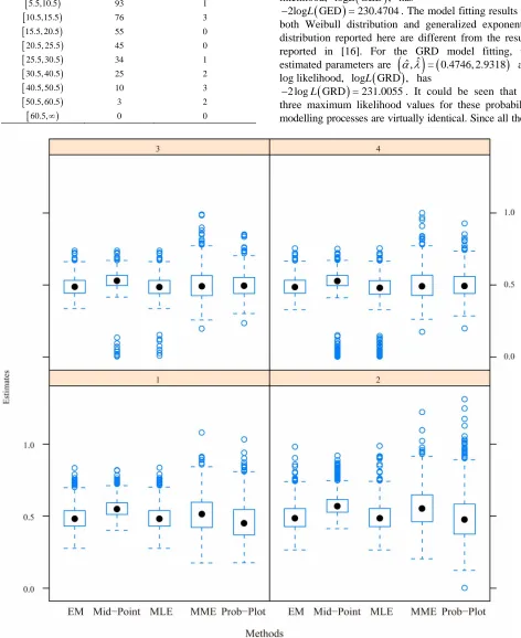
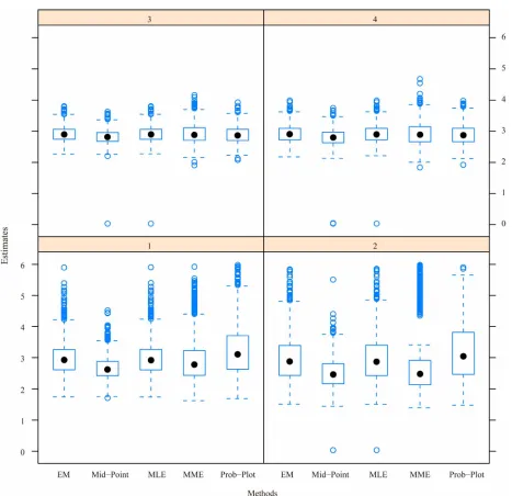
Figures 1 and 2 where the medians of the boxplots for the processes of the regular MLE and EM algorithm are close to the input population parameters,



 



= , = 0.48, 2.93

   , for the simulation study. However, the boxplots shows that almost all the plots are right skewed except the cases of the plots for the regular MLEs and the MLEs via midpoint approximation for  under the progressive interval censoring schemes of p_{ 3}

and p_{ 4} . The box plots also show potential outliers happened for many cases except the

ive censoring scheme p_{ 3}. It could be due to the convergence problem from the iterative process that outliers happen. Over all, from the box plots, we can conclude that process via E algorithm provides the best convergence results.

As e performances among the four censoring schemes, the third scheme p_{ 3} provides the most precise results as seen from “Bias”, “SD” (i.e the standard deviation) and “MSE” (i.e. the mean squared errors) shown in Table 1, then followed by the schemes

 4

p , p_{ }1 or p 2 . The results of the performance comparisons among these censoring schemes are

case from

M

th

.

similar

mete estim sho

for the maximum likelihood estimate, “M

EM algorithm under progress

to the results observed in [15] and [16]. These phe- nomena are expected since the third censoring scheme could have the largest number of failure items observed before the termination of life-testing and then followed by p_{ 4} , p_{ 1} and p_{ 2} . Intuitively, these are also

with statistical theory that the larger the “sample size” is the more accuracy the parameter estimate is.

Among these three estimators developed in the paper, the maximum likelihood estimator (via regular process and EM algorithm in the paper) gives the most precise para r ates as wn by SD and MSE in Table 1. Therefore, we recommend the maximum likelihood estimation. Among the three processes, “MLE” “MidPt” and “EM”,

consistent the

[image:8.595.61.538.95.413.2]

Y. L. LIO ET AL. 53

Table 1. Summary of simulations assuming both α and λ unknown.

 

Scheme EM MidPt MLE MME ProbPt EM MidPt MLE MME ProbPt

1 Median 0.481 0.548 0.481 0.514 0.451 2.926 2.622 2.921 2.780 3.109

2 Median 0.485 0.569 0.486 0.553 0.477 2.877 2.460 2.867 2.480 3.055

Me an 0

3 di .487 0.530 0.487 0.491 0.495 2.904 2.821 2.905 2.884 2.871

4 Median 0.486 0.528 0.481 0.492 0.494 2.908 2.803 2.906 2.894 2.878

1 Mean 0.488 0.555 0.488 0.514 0.462 2.990 2.671 2.990 2.987 3.289

2 Mean 0.494 0.580 0.495 0.549 0.496 2.985 2.421 2.976 2.850 3.275

3 Mean 0.490 0.529 0.486 0.500 0.500 2.912 2.802 2.889 2.918 2.890

4 Mean 0.491 0.521 0.476 0.504 0.502 2.917 2.746 2.848 2.920 2.894

1 Bias 0.008 0.075 0.008 0.034 0.018 0.060 0.258 0.060 0.057 0.359

2 Bias 0.014 0.100 0.015 0.069 0.016 0.055 0.509 0.046 0.080 0.345

3 Bias 0.010 0.049 0.006 0.020 0.020 0.018 0.128 0.041 0.012 0.040

4 Bias 0.011 0.041 0.004 0.024 0.022 0.013 0.184 0.082 0.010 0.036

1 SD 0.084 0.062 0.085 0.133 0.131 0.545 0.371 0.549 0.794 0.930

2 SD 0.095 0.080 0.097 0.153 0.173 0.742 0.720 0.765 1.256 1.898

3 SD 0.064 0.070 0.077 0.106 0.083 0.249 0.352 0.377 0.313 0.268

4 SD 0.067 0.096 0.098 0.110 0.091 0.291 0.528 0.560 0.372 0.314

1 MSE 0.007 0.009 0.007 0.019 0.018 0.304 0.205 0.300 0.633 0.993

2 MSE 0.009 0.016 0.010 0.028 0.030 0.553 0.777 0.588 1.584 3.722

3 MSE 0.004 0.007 0.006 0.012 0.007 0.062 0.140 0.144 0.098 0.074

4 MSE 0.005 0.011 0.010 0.013 0.009 0.085 0.312 0.320 0.138 0.100

4. R al Da

nal

4.1 he D

with plasma ell myeloma treated at the National Cancer Institute for modelling the two-parameter GRD. his data had been discussed in [15], [16] and [22]. To

ived at the right end of each tim

e

ta A

ysis

. T ata

A data set which consists of 112 patients c

(See [21]) is used T

be self-contained, the data are re-produced here in the

Table 2 for easy reference.

The most right side column in Table 2 shows the number of patients who were dropped out from the study at the right end of each time interval. These dropped patients are known to be surv

e interval but no follow-up. Hence, the most right side column in Table 2 provides the values of

, = 1, , = 9

i

R i  m . The number of failures,

, = 1, ,

i

X i  m, can be easily calculated to be





= 18,16,18,10,11,8,13, 4,1

X from the number at risk

and the number of withdrawals.

omparisons Weibull distribution from [15] a 4.2. Model C

nd generalized expon- ntial distribution from [16] have been used to model the

a cell m

C d 6] p e

lling sse een bul ibut d

generalized exponential distribution by using presche- h. Chen and Lio [16] indi- ted that the generalized exponential distribution pro- plasm yeloma data set with prescheduled times in terms of month. hen an Lio [1 also com are th mode proce s betw Wei l distr ion an

duled times in terms of mont ca

vided better model fit than the Weibull distribution does. In this paper, we would like to compare the modelling processes among Weibull distribution, generalized ex- ponential distribution and generalized Rayleigh distri- bution. To compare the modelling processes among these three distributions, the prescheduled times are converted into in terms of year. Here, it is for easy reference that the pdfs of Weibull distribution and generalized expon- ential distribution are given, respectively, below:





1





, , = exp , > 0, > 0, > 0, w

f t   t t x   (4.1) and

















1

GED , , = exp 1 exp ,

> 0, > 0, > 0.

f t t t

t



    

 



  

(4.2)

The model fitting to the classical Weibull distribution (1) yields the estimated parameters

 

 ˆ ˆ, = 0.447,1.23





and log likelihood, logL



WD ,



Table 2. Plasma cell myeloma survival times.

Interval in Months Number at risk Number of withdr

has

awals

0,5.5 112 1

5.5,10.5  93 1

10.5,15.5  76 3



15.5, 20.5 55

45

0 0

20.5, 25.5 

25.5, 30.5  34 1

30.5, 40.5 



25 2



5

40.5, 50. 10 3

50.5, 60.5  3 2

60.5, 0 0





2logL WD = 230. 1



the generalized exponentia mated parameters

340 and the model fitting to l distribution

esti

(2) has the

 

ˆ =

ihood,



1.433, 0.686



ˆ ,

 and log

likel logL



GED ,



has





2logL GED = 230.4704

 . The model fitting results for both Weibull distributi xponential distribution re are d

on ported here reported in [16]. For th

and generalized e

ifferent from the results e GRD model fitting, the estimated parameters are

 

 ˆ , ˆ = 0.4746, 2.9318





and log likelihood, logL



GRD ,



has





2 logL GRD = 231.0055

 . It could be seen that all

three maximum likelihood bility modelling proce ally ide

values for these proba sses are virtu ntical. Since all these

[image:9.595.55.527.124.702.2]

from 1000 simulations for the five estimation methods and four simulation schemes for α=0.48.

[image:10.595.67.534.70.522.2]

Y. L. LIO ET AL. 55

Figure 2. Boxplot for from 1000 simulations for the five estimation methods and four simulation schemes for

three distributions have no sub-model relationship, the chi-square test ca

a d

set. Although Kundu and Raqab [5] and Raqab and Kundu [7] had detail comparison among these distribution for a random sample, statistical inference to discriminate among these distributions has not been developed for the progressively type-I interval censored data, yet. Therefore, a more detail comparison among these three distributions under progressive type-I interval censoring is not available according to our best know- ledge.

To apply the Kolmogorov-Smironov goodness-of-fit test for fitting a given complete data set with a dis-

tribution,

λ λ=2.93 .

n not be applied directly to select mong these three mo els for modeling the given data

 

F x , the maximum distance,

 

= sup0 < ˆ

 

 

ˆ

n x n

D F _{ } F x F x , between the empirical distribution, Fˆn

 

x , of the given data set and the population distribution, F x

 

ˆ with ˆ as the

MLE of , must be obtained. When a progressively censore is given, the empirical distribution is replaced b the product-limit distribution defined through E ion (19) in the formula . Fitting the give a set with the Weibull di

d data y quat n dat

 

n

D F

stribution Fw,

 

.15737

n w

D F = 0 , with the GE distribution FGED,



GED



= 0.1618

n

D F and with the GRD FGRD,



GRD



= 0.1708

n

Kolmogorov-Smironov goodness-of-fit test for the Wei- bull distribution and generalized exponential distribution are different from the reports of [16]. The sampling distribution of should have been applied to find the critical val e goodness-of-fit tests mentioned. Although the ling distribution for under any progre ing has not been d, we can see that no gnificant differe these three numerical

5. Discussio s and Conclusions

In this paper, t thods to estim ters of the two-para neralized Rayleigh bution under progress nterval censori n de- veloped. They mum likelihood est on, esti- mation of me ents and the estim d on the probability plot.

The simu in the case of mode large size data set i regular MLE and m ximum

algorithm relatively more accurate ter estimation an ximum likelihood estimate via EM algorithm ost precise estima ummarized in the and

Figures 1 and therefore recom EM

algorithm proc be used to estima eters in the GRD un essive type-I interval ng.

The develo are also applied t data which contains 112 patients with plasma eloma Institute to demonstrate the applicabilit the process of GRD m

found that the of likelihood functi ses to zero when the duled times in term onth and the estima eters are senstive to the initial parameter inputs for iterative proce rescales for the presch es have been trie found

that the presc es mu nto in

t

ropulation pa ter estimations. The ter esti-

pone n and gene yleigh

di

difference among these three modelling processes. Hence, the discriminate process among these three distibutions under progressive type-I censoring could be an important future research.

6. Acknowledgements

The authors would like thank to the editor and anony- mous referees for their suggestions and comments, which significantly improved this manuscript.

7. References

[1] I. W. Burr, “Cumulative Frequency Distribution,” Annual of Mathematical Statistics, Vol. 13, No. 2, 1942, pp. 215-232.

[2] K. E. Ahmad, M. E. Fakhry and Z. F. Jaheen, “Empirical Bayes Estimation of P (Y < X) and Characterization of Burr-Type X Model,” Journal of Statistical Planning and Inference, Vol. 64, No. 2, 1997, pp. 297-308.

doi:10.1016/S0378-3758(97)00038-4

 

n

D F

ue for th samp ssive censor

any si reports.

n

hree me meter ge

ive type-I i are maxi thod mom

lation study ndicates that likelihood estimate via EM

parame

tion as s

2. We ess to der progr ped methods

treated at the National Cancer y. In

value presche tions of param

eduled tim heduled tim

rame

ntial distributio

 

n

D F

develope nce among

ate the parame distri ng have bee

imati ation base

rate a gives

d the ma produces the m

Table 1

mend the te the param

censori o a real cell my

odelling, it is on (2.2) clo

s of m

sses. Many d. We st be converted i

parame

ralized Ra

[3] Z. F. Jaheen, “Bayesian Approach to Prediction with Outliers from the Burr Type X Model,” Microeleclron Reliability, Vol. 35, No. 4, 1995, pp. 45-47.

doi:10.1016/0026-2714(94)00056-T

[4] Z. F. Jaheen, “Empirical Bayes Estimation of the Reli-ability and Failure Rate Functions of the Burr Type X Failure Model,” Journal Applied Statistical Science, Vol. 3, No. 2, 1996, pp. 281-285.

[5] D. Kundu and M. Z. Raqab, “Generalized Rayleigh Dis-tribution: Different Methods of Estimation,” Computa-tional Statistics and Data Analysis, Vol. 49, No. 1, 2005, pp. 187-200. doi:10.1016/j.csda.2004.05.008

[6] M. Z. Raqab, “Order Statistics from the Burr Type X Model,” Computational Mathematical Applications, Vol. 36, No. 4, 1998, pp. 111-120.

doi:10.1016/S0898-1221(98)00143-6

[7] M. Z. Raqab and D. Kundu, “Burr Type X Distribution: Revisited,” 2003.

Predicti

e cation in

tics: Theo , 1991, pp.

2307-2330. doi:10.1080/0361092

erms of year to produce better convergence results in the p

mates for the GRD via EM algorithm and regular MLE are quite similar. This real data set modelling confirms the results observed from the simulation study.

Since the GRD was introduced for lifetime data, this study was the first time to introduce the progressive type-I interval censoring to the GRD based on our best knowledge. We believe that this study contributes to the literatures and the research community in this lifetime data analysis for the generalized Rayleigh distribution as well as for progressive type-I interval censoring.

The comparison among Weibull distribution, genera- lized ex

stribution in the modelling process for the progre- ssively type-I interval censored data shows that no much

http://home.iitk.ac.in/ kundu/paper118.pdf

[8] H. A. Sartawi and M. S. Abu-Salih, “Bayes on Bounds for th Burr Type X Model,” Communi Statis ry and Methods, Vol. 20, No. 7

9108830633

[9] J. Q. Surles and W. J. Padgett, “Inference for P(Y < X) in del,” J

pp.

225-[10] J. Q. Surles and W. J. Padgett, “Inference for Reliability the Burr Type X Mo ournal Applied Statistical Sci-ence, Vol. 7, No. 2, 1998, 238.

and Stress-Strength for a Scaled Burr Type X Model,”

Lifetime Data Analysis, Vol. 7, No. 2, 2001, pp. 187-200.

doi:10.1023/A:1011352923990

[11] J. Q. Surles and W. J. Padgett, “Some Properties of a Scaled Burr Type X Model,” Joournal Statisticsal

Plan-8 -200.

ning and Infere 7

[12] N. L. Johnson, S nan, “Continuous Univariate Distr John Wiley

Y. L. LIO ET AL. 57

0.

Inf

istribution Based on Progressively

rnal of Statistical

009, pp. 145-159. doi:10.1080/00949650701648822

and Sons, New York, 1995.

[13] N. Balakrishnan and R. Aggarwala, “Progressive Cen-soring: Theory, Methods and Applications,” Birkha User, Boston, 200

[14] R. Aggarwala, “Progressively Interval Censoring: Some Mathematical Results with Application to erence,”

Communications in Statistics-Theory and Methods, Vol. 30, No. 8, 2010, pp. 1921-1935.

[15] H. Ng and Z. Wang, “Statistical Estimation for the Pa-rameters of Weibull D

type-I Interval Censored Sample,” Jou

Computation and Simulation, Vol. 79, No. 2, 2

[16] D. G. Chen and Y. L. Lio, “Parameter Estimations for Generalized Exponential Distribution under Progressive Type-I Interval Censoring,” Computational Statistics and Data Analysis, Vol. 54, No. 6, 2010, pp. 1581-1591.

doi:10.1016/j.csda.2010.01.007

[17] A. P. Dempster, N. M. Laird and D. B. Rubin, “Maxi-mum Likelihood from Incomplete Data via the EM

Algo-rithm,” Journal of the Royal Statistical Society: Series B, Vol. 39, No. 1, 1977, pp. 1-38.

[18] R Development Core Team, “A Language and Environ-ment for Statistical Computing,”R Foundation for Statis-tical Computing,Vienna, 2006.

an, “R: A Language for Data Analysis and graphics,” Journal of Computational and

[19] R. Ihaka and R. Gentlem

Graphical Statistics, Vol. 5, No. 3, 1996, pp. 299-314.

doi:10.2307/1390807

[20] C. D. Kemp and W. Kemp, “Repid Generation of Fre-quency Tables,” Applied Statistics, Vol. 36, No. 3, 1987,

oi:10.2307/2347786

pp. 277-282. d

L. E. Kellerhouse and E. A. Gehan,

“Plas-ol. 42, No. 6, 1967, pp. 937-948. [21] P. P. Carbone,

macytic Myeloma: A Study of the Relationship of Sur-vival to Various Clinical Manifestations and Anomalous Protein Type in 112 Patients,” The American Journal of Medince, V

doi:10.1016/0002-9343(67)90074-5