Relations among partitions

R. A. Bailey

Abstract

Combinatorialists often consider a balanced incomplete-block design to consist of a set of points, a set of blocks, and an inci-dence relation between them which satisfies certain conditions. To a statistician, such a design is a set of experimental units with two partitions, one into blocks and the other into treatments; it is the relation between these two partitions which gives the design its prop-erties. The most common binary relations between partitions that occur in statistics are refinement, orthogonality and balance. When there are more than two partitions, the binary relations may not suffice to give all the properties of the system. I shall survey work in this area, including designs such as double Youden rectangles.

1

Introduction

Many combinatorialists think of a balanced incomplete-block design (BIBD) as a set P of points together with a collection B of subsets of P, called blocks, which satisfy various conditions. For example, see [52]. Some papers, such as [16, 65, 199], call a BIBD simply adesign. Others think of it as the pair of sets P and B with a binary incidence relation between their elements. These views are both rather different from that of a statistician who is involved in designing experiments. The following examples introduce the statistical point of view, as well as serving as a basis for the combinatorial ideas in this paper.

Example 1.1 A horticultural enthusiast wants to compare three varieties of lettuce for people to grow in their own gardens. He enlists twelve peo-ple in his neighbourhood. Each of these prepares three patches in their vegetable garden, and grows one of the lettuce varieties on each patch, so that each gardener grows all three varieties.

Here the patches of land are experimental units. There may be some differences between the gardeners, so the three patches in a single garden form what is called ablock. Each variety occurs just once in each block, and so the blocks are said to becomplete. Complete-block designs were advocated by Fisher in [78], and are frequently used in practice.

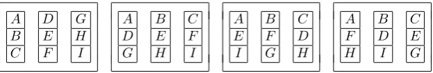
A B C D E F G H I A D G B E H C F I A E I B F G C D H A F H B D I C E G

Figure 1: Balanced incomplete-block design in Example 1.2: columns rep-resent blocks and letters reprep-resent varieties

grow nine different varieties, so each gardener still uses only three patches of ground, and thus can grow only three varieties. The blocks are now incomplete, in the terminology of Yates [225].

One possible layout is shown in Figure 1. This incomplete-block design has the property that each pair of distinct varieties concur in the same number of blocks (here, exactly one). Yates originally called incomplete-block designs with this propertysymmetrical, but the adjective had been changed tobalanced within a few years [46, 80].

To a statistician, the partition of the set of experimental units into blocks is inherent and is known before the decision is taken about which variety to allocate to each unit. This allocation gives another partition of the set of experimental units, and it is the relation between these two partitions that is regarded as balance. It is not a symmetric relation, in general. In Example 1.2 the varieties are balanced with respect to the blocks, but the blocks are not balanced with respect to the varieties because some pairs of blocks have one variety in common while others have none. This relation is discussed in more detail in Section 5.

In fact, statisticians usually call these partitions factors, because the names of the parts are relevant. In Example 1.2 the names of the varieties are not interchangeable; we probably want to find out which one does best. Thus a factor is typically regarded as a function from the set of experimental units to a finite set: ifB andLdenote the factors for blocks and lettuce varieties respectively and ω is a vegetable patch then B(ω) is the block (garden) containingω and L(ω) is the variety grown on ω. Furthermore,|B(ω)|is the size of the block containing ω, while|L(ω)|is the number of patches with the same variety as that grown onω.

A response Yω, such as total yield of edible lettuce in kilograms, is

measured on each patch ω. It is usually assumed that Yω is a random

variable and that there are constantsτi andβj such that

Yω=τL(ω)+βB(ω)+εω, (1.1)

where the final termsεωare independent random variables with zero mean

dis-A B C D E F G H I A D G B E H C F I A E I B F G C D H A F H B D I C E G

Figure 2: Resolved balanced incomplete-block design in Example 1.3: columns represent blocks, rectangles represent districts and letters rep-resent varieties

tributed. The purpose of the experiment is to estimate the constants τi.

Of course, this is impossible, because equation (1.1) is unchanged if a con-stant is added to every τi and subtracted from every βj, but we aim to

estimate differences such as τ1−τ2, that is, to estimate theτi up to an

additive constant.

Thus the two partitions have different roles. One (the partitionB) is inherent, and we are usually not interested in the effectsβjof the different

parts. The other (the partition L) has its parts allocated by the experi-menter, and the purpose of the experiment is to find out what differences there are between its parts. Nonetheless, this paper will concentrate on the combinatorial relation between them. Before doing so, we give some examples with three partitions.

Example 1.3 Suppose that the twelve gardeners in Example 1.2 do not all live in the same neighbourhood. Instead, they are spread over four dif-ferent districts, with three per district. If the first three blocks in Figure 1 represent the gardens in the first district, and so on, then each variety is grown once in each district, as shown in Figure 2. This is convenient if other people want to look at the different varieties during the course of the experiment.

Each block is contained within a single district, so the partition into blocks is arefinement of the partition into districts. Section 3 discusses refinement in more detail. On the other hand, the partitions into districts and into varieties have the property that each part of one (a district) meets each part of the other (a variety) in a single experimental unit. This is a special case ofstrict orthogonality, which is explained in Section 4.

The assumption aboutYω might remain as in (1.1) or it might be

Yω=τL(ω)+βB(ω)+γD(ω)+εω, (1.2)

where D(ω) is the district containing ω. Of course, if the βj and γk are

A B C D E F G C D E F G A B D E F G A B C E F G A B C D

Figure 3: Row–column design in Example 1.4: rows represent months, columns represent people and letters represent exercise regimes

to γ1 and subtract it from βj for all blocks j in district 1. However, it

is sometimes assumed that theβj are independent random variables with

zero mean and the same variance σ2

B. Section 6.2 discusses further the

potential difficulty in an assumption like (1.2) when one partition is a refinement of another.

An incomplete-block design whose blocks can be grouped into collec-tions each of which contains each variety just once, as in Example 1.3, is calledresolvable. Section 15 gives more information about such designs.

Example 1.4 In order to assess the benefits of different exercise regimes, a health scientist asks seven healthy people to participate in an experiment over four months. Each month each person will be allocated one of seven exercise regimes. At the end of each month, the change in some measure of fitness, such as heart rate, will be recorded for each person.

Now each experimental unit is one person for one month. The parti-tions into months and into people are inherent, but the scientist chooses the partition into exercise regimes. Figure 3 shows one possible design for this experiment. The partitions into months and into people are strictly orthogonal to each other, as are the partitions into months and into ex-ercise regimes. The partitions into people and into exex-ercise regimes are both balanced with respect to each other.

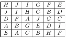
Example 1.5 A small modification of Example 1.4 has five months, six people and ten exercise regimes. One possible design is shown in Fig-ure 4, where rows represent months, columns respresent people and letters represent exercise regimes.

H J I G F E

J I H C B D

D F A J G C

A B G E D I

E A C B H F

Figure 4: Combinatorial design used in Examples 1.5 and 1.6

Denote by R, C and L the partitions into rows, columns and letters in the design in Figure 4. From the point of view of the statistician, the uses of this design in Examples 1.5 and 1.6 are quite different. In the former, the partitionsRandCare inherent whileLis at the choice of the experimenter; in the latter,L is inherent while the experimenter chooses

RandC. However, in both cases it may be assumed that

Yω=αR(ω)+φC(ω)+τL(ω)+εω. (1.3)

From a combinatorial point of view, Figure 4 simply shows a set with three partitions. The partitions R and C are strictly orthogonal to each other, while each ofR andC is balanced with respect to letters. In fact, there is a third property, calledadjusted orthogonality, that will be defined in Section 8.

For further explanation of how combinatorial design problems arise from statistically designed experiments, see [22, 33, 177, 202].

The remainder of this paper treats a combinatorial design as a collec-tion of particollec-tions of a finite set. Seccollec-tion 2 establishes some notacollec-tion for partitions and their associated matrices and subspaces. Sections 3–5 dis-cuss the three most important binary relations between partitions, all of which have been seen in the examples so far. Section 6 explains more about the background to equations (1.1)–(1.3). Section 7 discusses the relations between the subspaces defined by partitions, and shows that sometimes there is a need for a ternary relation. Sections 8 and 9 give more details of two important non-binary relations. These are used in Section 10, which considers possibilities for three partitions. This leads to several different types of combinatorial design, considered in the remaining sections. Each type is defined by three partitions, or is a simple generalization with more partitions but no need for any further non-binary relations.

2

Partitions on a finite set

partitions of Ω.

IfF is such a partition, denote bynF its number of parts. Thee×nF

incidence matrix XF has (ω, i)-entry equal to 1 if unitω is in partiofF;

otherwise, this entry is zero. ThusX_FX_F> is thee×erelation matrix for

F, with (ω1, ω2)-entry equal to 1 ifω1 andω2 are in the same part ofF,

and equal to 0 otherwise. ThenF×nF matrixXF>XF is diagonal, with

(i, i)-entry equal to the size of the i-th part ofF.

Definition A partition isuniform if all of its parts have the same size.

Many statisticians, including Tjur [206, 207], call uniform partitions balanced, but this conflicts with the notion of balance introduced in Sec-tion 1. This terminology is discussed again in SecSec-tion 9. Preece reviewed the overuse of the word balance in design of experiments in [155]. The adjectiveshomogeneous [44],proper [151] andregular [66] are also used.

IfF is uniform, denote the size of all its parts bykF. ThennFkF =e

andX_F>X_F =kFInF, whereIn is the identity matrix of ordern.

Denote byRΩthe real vector space of dimension ewhose coordinates are labelled by the elements of Ω, so that each vector may be regarded as a function from Ω toR. IfF is a partition of Ω, denote byVF the subspace

ofRΩ _{consisting of vectors which are constant on each part of F. Then}

dim(VF) =nF.

We assume the standard inner product on RΩ_{. Denote by P} F the

matrix of orthogonal projection ontoVF. ThenPFreplaces the coordinate

yω of any vectory by the average value of yν forν inF(ω), which is the

part ofF containingω. In fact,PF =XF X

>

FXF

−1

X_F>. IfF is uniform thenX_FX_F>=kFPF.

Equations (1.1)–(1.3) all have the form

Y = X

F∈F

XFψF+ε, (2.1)

whereY andεare random vectors of lengthe,Fis a set of partitions of Ω, and, forF in F, ψF is a real vector of length nF. Thus the expectation

E(Y) ofY is in the subspacePF∈FVF.

There are two trivial partitions on Ω, which are different whene >1. The parts of the equality partition E are singletons, so kE = 1, nE =e

andXE =Ie=PE. At the other extreme, the universal partition U has

a single part, so nU = 1, kU =e, XUXU> =Jee and PU =e−1Jee, where

Jnmdenotes then×mmatrix with all entries equal to 1. Moreover,VEis

the whole space RΩ, whileVU is the 1-dimensional subspace of constant

IfFandGare two partitions of Ω, theirnF×nGincidence matrixNF G

is defined byNF G=XF>XG. The (i, j)-entry is the size of the intersection

of thei-th part ofF with thej-th part ofG. In particular,NEF =XF.

Given a setFof partitions of Ω, denote byAF the algebra ofe×ereal matrices generated by the projection matricesPF forF inF, and denote

byJF the algebra generated by the relation matrices XFXF> forF in F.

These are the same if all partitions inF are uniform. James calledJF the relationship algebraofF in [99], but it was shown in [100, 115] thatAF is more useful for understanding the properties ofF relevant to a designed experiment.

3

Refinement

Definition IfF andGare partitions of Ω, thenF isfinerthanG (equiv-alently, G is coarser than F) if every part of F is contained in a single part of Gbut at least one part of Gis not a part of F. This relation is denotedF ≺Gor GF.

In Example 1.3,B≺D. IfF≺GthennF > nG andVG< VF.

WriteF ₄G(orG_<F) to mean that eitherF ≺Gor F =G. Then 4is a partial order. For every partitionF, it is true thatE₄F ₄U and

VU ≤VF ≤VE.

Proposition 3.1 LetF andGbe partitions ofΩ. IfF ₄GthenPFPG=

PGPF =PG.

As with any partial order, there is a choice about which of the two objects should be considered ‘smaller’. Some statisticians write the refine-ment partial order in the opposite way to that used here. For example, see [31, 206, 207].

Since there are only a finite number of partitions of Ω, there is no difficulty with the next definition.

Definition Let F and G be partitions of Ω. The infimum F ∧G of

F and G is the coarsest partition H satisfying H ₄ F and H ₄ G; its parts are the non-empty intersections of a part of F and a part of G. Thus F ∧G = E if and only if no part of F intersects any part of G

in more than one unit. The supremum F ∨G of F and G is the finest partition K satisfying F ₄ K and G ₄ K; its parts are the connected components of the graph with vertex-set Ω and an edge between ω1 and

Thus if F ₄ G then F ∧G = F and F ∨G = G. In the design in Figure 4,R∧C=R∧L=C∧L=E andR∨C=R∨L=C∨L=U.

Proposition 3.2 If F andGare partitions ofΩthen VF ∩VG=VF∨G.

4

Orthogonality

4.1 Definitions

As Preece noted in [154], the wordorthogonalhas many different mean-ings in the statistical literature. Here I use the terminology in [23, 25, 32, 206].

Proposition 3.2 shows that subspacesVF andVG can never be

orthog-onal to each other. This motivates the following definition, from [206].

Definition Let V and W be subspaces of RΩ_{. Then V and W are}

geometrically orthogonalto each other if the subspacesV ∩(V∩W)⊥and

W∩(V ∩W)⊥ are orthogonal to each other.

Proposition 4.1 Let F and G be partitions of Ω. The following state-ments are equivalent:

(i) VF is geometrically orthogonal toVG;

(ii) PFPG=PGPF;

(iii) PFPG=PF∨G;

(iv) for every unitω, we have|F(ω)| |G(ω)|=|(F∧G)(ω)| |(F∨G)(ω)|.

The second statement above is sometimes called ‘projectors commute’, and the fourth ‘proportional meeting within each class of the supremum’.

Definition Let F and G be partitions of Ω. ThenF is orthogonal to

G, written F ⊥G, if PFPG =PGPF; and F is strictly orthogonal to G,

writtenF⊥G, ifPFPG=PGPF =PU.

Duquenne calls these two conceptslocal orthogonalityandorthogonality respectively in [66]; the latter agrees with Gilliland’s definition of orthog-onality in [83]. Some authors split the definitions further according to whether or notF∧Gis uniform.

A B B C A C

C A B

Figure 5: A 2×3 row–column design with nine units and three letters, giving mutually orthogonal partitions into rows, columns and letters

Figure 6: Two blocks, each of which is a 3×4 rectangle, so that there are 6 rows and 8 columns

In the design in Figure 4, R⊥C. IfR,C and Ldenote the partitions into rows, columns and letters in Figure 5, thenR⊥C,R⊥LandC⊥Leven thoughR, R∧C and R∧L are not uniform, because the ‘proportional meeting’ condition in Proposition 4.1(iv) is satisfied for all pairs and all pairwise suprema are equal toU. IfB,RandCdenote the partitions into blocks, rows and columns in Figure 6, thenR ⊥C but R is not strictly orthogonal toCbecause R∨C=B 6=U.

Proposition 4.2 LetF andGbe partitions ofΩ. ThenF⊥Gif and only ifNF G =e−1(XF>XF)JnFnG(X

>

GXG).

4.2 Orthogonal arrays

Definition An orthogonal array of strength two on Ω is a collection F of at least two uniform partitions of Ω with the property that every pair of distinct partitions is strictly orthogonal. Inductively, form ≥ 3, a collection F of at least m partitions of Ω is an orthogonal array of strength mif it is an orthogonal array of strength m−1 and, whenever

F1, . . . ,Fmare distinct partitions inF, the infimumF1∧F2∧ · · · ∧Fm−1

is strictly orthogonal toFm.

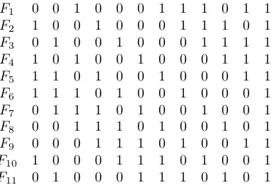
Figure 7 shows an orthogonal array of strength two withe= 12,|F |= 11, andnF = 2 for all F in F. It is equivalent to that given by Plackett

F1 0 0 1 0 0 0 1 1 1 0 1 1

F2 1 0 0 1 0 0 0 1 1 1 0 1

F3 0 1 0 0 1 0 0 0 1 1 1 1

F4 1 0 1 0 0 1 0 0 0 1 1 1

F5 1 1 0 1 0 0 1 0 0 0 1 1

F6 1 1 1 0 1 0 0 1 0 0 0 1

F7 0 1 1 1 0 1 0 0 1 0 0 1

F8 0 0 1 1 1 0 1 0 0 1 0 1

F9 0 0 0 1 1 1 0 1 0 0 1 1

F10 1 0 0 0 1 1 1 0 1 0 0 1

F11 0 1 0 0 0 1 1 1 0 1 0 1

Figure 7: Orthogonal array of strength two, consisting of 11 partitions of a set of size 12 into two parts: columns represent elements of the set, and each row shows one partition

Forn≥2, the rows, columns and letters of any Latin square of ordern

give an orthogonal array of strength two on a set of size n2_{, with three}

partitions into parts of sizen. See [95] for many uses and constructions of orthogonal arrays, as well as more theory. Eendebak and Schoen maintain a catalogue on the web page [76].

From Finney [77] onwards, finite Abelian groups have been a fruitful source of orthogonal arrays, under the name fractional factorial designs. Fori = 1, . . . , slet Gi be an Abelian group of orderni, where ni ≥ 2.

Let G be the product group G1×G2× · · · ×Gs. Every complex

irre-ducible characterχ ofGhas the formχ= (χ1, χ2, . . . , χs) whereχi is an

irreducible character ofGi andχ(g1, g2, . . . , gs) =χ1(g1)χ2(g2)· · ·χs(gs).

LetH be a subgroup ofG, and letFi be the partition ofH defined by the

values of thei-th coordinate. Then{F1, . . . , Fs}forms an orthogonal array

of strengthmonH if and only if the only non-trivial charactersχon G

whose restriction toH is trivial have non-trivial componentsχifor at least

m+ 1 values ofi. For example, ifs= 3, n1=n2 =n3= 7 and Gi isZ7

written additively fori= 1, 2 and 3 then{F1, F2, F3}forms an orthogonal

array of strength two on the subgroupH ={(g1, g2, g3) :g1+g2+g3= 0}.

Up to isotopism (permutations of the names of the parts of each partition), this is the Latin square obtained as the Cayley table ofZ7.

Some papers, such as [61, 112, 141, 213], call an orthogonal array reg-ular if and only if it is made from an Abelian group in this way. There are two problems with this. The first is that, in each experiment, the parts ofFi (such as varieties of lettuce) are unlikely to be labelled by the

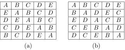
A B C D E

E A B C D

D E A B C

C D E A B

B C D E A

A B C D E

B A D E C

E D A C B

C E B A D

D C E B A

(a) (b)

Figure 8: Two Latin squares of order five: square (a) is isotopic to the Cayley table ofZ5, but square (b) is not

data to know whether or not the orthogonal array was constructed from Abelian groups? In any case, this derivation makes no difference to the data analysis. The second problem is that, for an experiment designed using a Latin square, it is usually of no practical importance whether or not the square is isotopic to the Cayley table of an Abelian group. Asn

increases, so does the proportion of Latin squares of ordernwhich are not isotopic to such Cayley tables. Figure 8 shows two Latin squares of order five: only one of them is isotopic to a Cayley table.

The definitions in this section show that, in an orthogonal array F of strength two, PF commutes with PG for all F and G in F.

Propo-sition 4.1 shows that commutativity cannot be destroyed by inclusion of suprema. Thus Gr¨omping and Bailey, in their paper [86] giving some more lenient definitions of regularity, proposed calling an orthogonal array geo-metrically regular if PG1∧···∧Gr commutes withPH1∧···∧Hs for all subsets {G1, . . . , Gr} and {H1, . . . , Hs} of F. Thus the two orthogonal arrays in

Figure 8 are geometrically regular, while the one in Figure 7 is not, because

F1∧F2 is not orthogonal toF3.

4.3 Tjur block structures and orthogonal block structures

Proposition 4.1 leads to these definitions, given in [23], building on the work in [206].

Definition Let F be a set of partitions on a finite set Ω. Then F is a Tjur block structure ifF is closed under taking suprema, every pair of partitions inFis orthogonal, andE∈ F. If, in addition,Fis closed under taking infima, every partition inF is uniform, and U ∈ F, thenF is an orthogonal block structure.

ForF inF, define a further subspaceWF ofRΩby

WF =VF ∩

\

F≺G∈F

VG⊥=VF∩

X

F≺G∈F

VG

!⊥

.

Theorem 4.3 If F is a Tjur block structure then the subspacesWF, for

F inF, are mutually orthogonal and their sum is RΩ_.

It follows that the dimensions of the subspacesWF, and the matrices

of orthogonal projection onto them, can be calculated recursively, starting with the coarsest partition inF. Moreover, the algebraAF is commuta-tive, and consists of all real linear combinations of the matricesPF, for

F in F. The subspacesWF are the mutual eigenspaces of AF. For any

partition inF which is uniform, its relation matrix is also inAF.

Tjur block structures are used widely in statistics, in two different contexts, which are explained more in Section 6. One concerns covariance, and the other expectation.

The covariance cov(Yα, Yβ) of responses Yα and Yβ is defined to be

E[(Yα−E(Yα))(Yβ−E(Yβ))]. The variance-covariance matrix Cov(Y) of

the random vectorY in equation (2.1) is the e×ematrix whose entry in rowαand columnβis cov(Yα, Yβ). It is often assumed that Cov(Y) is an

unknown matrix inJHfor a specified Tjur block structureHwithH ⊆ F. If the partitions are all uniform thenJH =AH and so the eigenspaces of Cov(Y) are known. Then closure under suprema ensures that there is no pre-determined linear dependence among the eigenvalues, which avoids complications in estimating their values: see [35].

The other use is to give a collection of models for the expectation_E(Y) ofY. It is assumed, as in equations (1.1)–(1.3), that there is a subset G ofF such thatE(Y)∈PG∈GVG, and we would like to find the smallest

suchG: see [28]. Closure under suprema is essential for the existence of such a smallest subset.

The set of partitions{E, R, C, L, U} in any Latin square forms an or-thogonal block structure. Apart from Latin squares, and sets of mutually orthogonal Latin squares, most orthogonal block structures in common use are poset block structures, described in the next subsection.

4.4 Poset block structures

a Latin square into rows, columns and letters respectively, then standard analysis of variance in the popular statistical software R [175] can recog-nise that R∧C ₄ R and R∧C ₄ C but not that R∧C ₄L; nor can it recognise that H ₄ R if H is another name for the partition R∧C. Each software has its own symbol for the binary operator “∧”, usually something like “.” or “:” that is available on standard keyboards. The usual rule seems to be that A1∧A2∧ · · · ∧An is recognised to be finer

thanB1∧B2∧ · · · ∧Bmif and only if{B1, B2, . . . , Bm}is a proper subset

of{A1, A2, . . . , An}. This rule is true for so-called poset block structures

when their partitions are named canonically.

The definition of poset block structures needs another partial order, which I shall write as v. If (P,v) is a partially ordered set (poset for short), a subsetQofP is defined to beancestral, or anup-set, if whenever

i∈ Qandj∈ P withi<j thenj ∈ Q.

Definition Let P = {1, . . . , s} be a finite set with a partial order v. For i = 1, . . . , s, let Ωi be a finite set of size ni, where ni ≥ 2. Put

Ω = Ω1×Ω2× · · · ×Ωs. LetFi be the partition of Ω defined by the values

of thei-th coordinate, fori= 1, . . . , s. IfQ ⊆ P, define the partitionFQ of Ω byFQ =Vi∈QFi. Theposet block structure on Ω defined by (P,v)

is{FQ:Qis an ancestral subset ofP}.

Example 4.4 IfP ={1,2,3}with 1=2 and 1=3 then the correspond-ing poset block structure may be visualized asn1rectangles (parts ofF{1}) each defined byn2rows (parts ofF{1,2}) andn3columns (parts ofF{1,3}). Figure 6 shows an example withn1= 2, n2= 3 andn3= 4.

Example 4.5 Extend Example 1.4 so that there are 14 people, of whom seven are men and seven are women. If we ignore the partition into exercise regimes, we have the poset block structure defined by{1,2,3}withn1= 2,

n2= 7, n3= 4 and 2<1. The parts of F{1} are the genders; the parts of

F{1,2}are the people; the parts ofF{3}are the months; each part ofF{1,3} is one gender for one month; and the parts ofF{1,2,3} are the units.

Theorem 4.6 The following statements hold for any poset block structure defined by a poset(P,v).

(i) IfQ is an ancestral subset of P, then FQ is uniform, with all parts of size Q

i∈P\Qni.

(ii) The subsets ∅ and P are both ancestral. Moreover, F∅ = U and

(iii) IfQandRare both ancestral subsets ofP, thenFQ⊥FR,FQ∨FR=

FQ∩R andFQ∧FR=FQ∪R.

It follows that every poset block structure is an orthogonal block struc-ture. Latin squares show that the converse is not true.

Poset block structures were investigated extensively (but not so named) by Yates [224] and later by Kempthorne and his colleagues [107, 205, 232], but these authors did not manage to completely distinguish between the two partial orders involved. By restricting himself to series-parallel posets, Nelder was able to provide recursive definitions and constructions in [126] for what he called simple orthogonal block structures. This approach led to algorithms that underlie many different programs used today for the analysis of variance. Speed and Bailey pointed out in [197, 198] that Nelder’s approach can be used for arbitrary finite posets. Further details and examples are in [23, 26, 30].

5

Balance

In this section we denote byB andLtwo partitions of Ω whose parts will be calledblocks andletters respectively.

Definition The relationship betweenLandBisbinaryifL∧B=E; this means that each letter occurs at most once in each block. It isgeneralized binary if no two intersections of a part ofLwith a part ofB differ in size by more than one.

Confusion alert! The first of these really is a binary relation whose name is ‘binary’.

Ann×nmatrix is calledcompletely symmetric if it is a linear combi-nation ofIn andJnn.

5.1 Combinatorial notions of balance

Let i and j be two letters, not necessarily distinct. The number of ordered pairs (ω1, ω2) in Ω×Ω with the properties that B(ω1) =B(ω2),

L(ω1) = i and L(ω2) = j is equal to the (i, j)-entry of NLBNBL. It is

called theconcurrence ofiandj in blocks.

The classical definition of balance, given by Yates in [225], follows.

Definition If the partitionB is uniform andL∧B=E then the parti-tionLisbalancedwith respect toBif the off-diagonal elements ofNLBNBL

For a binary design, a counting argument shows that ifL is balanced with respect to B then L is also uniform and hence that NLBNBL is

completely symmetric. This definition of balance includes as a special case complete-block designs. In these, L is uniform, nBnL = e, NLBNBL =

nBJnLnL andL⊥B. For all other designs which are balanced according to this definition, the coefficient ofInL inNLBNBLis non-zero and therefore

NLBNBL has ranknL.

Fisher proved his famous inequality in [79]: ifL∧B=E,Bis uniform, andLis balanced with respect toB but not orthogonal toB, thennL ≤

nB. There are now many proofs of this result. One of the simplest is the

observation that the rank ofNLBNBLcannot be greater than the number

of columns ofNLB. Conversely, ifNLBNBL has ranknLandnL=nB, it

follows thatNLB is invertible: hence ifNLBNBLis completely symmetric

then so is NBLNLB and therefore B is also balanced with respect toL.

See [52, Chapter 1] and [202, Chapter 2].

How should this definition be generalized if B is not uniform or the relationship between L and B is not binary? Relaxing the uniformity ofB givespairwise balanced designs, introduced in [110]. Now a counting argument shows that the entries on the diagonal ofNLBNBLare all strictly

bigger than the common off-diagonal entry, and so NLBNBL is positive

definite; therefore it has ranknL, and Fisher’s inequality follows as before.

As [223] shows, pairwise balanced designs have been a very fruitful field of research, which includes results about the existence of BIBDs. However, as we show in the next subsection, this notion of balance does not match what is needed from the statistical point of view.

5.2 Statistical notions of balance

The vector form of equation (1.1) isY =XBβ+XLτ+ε. To estimate

the vector τ up to an additive constant, it is necessary to project the data vector onto the subspace (VL+VB)∩VB⊥. ThenL×nLinformation

matrix CLB is defined byCLB =XL>(Ie−PB)XL. Note thatIe−PB is

the matrix of orthogonal projection ontoV_B⊥. Also, ifB is uniform then

X_L>P_BX_L=k_B−1N_LBN_BL.

The matrix CLB is symmetric, with row-sums zero, so it is singular.

IfB ₄L then it is impossible to estimate any difference τi−τj. In this

case,CLB = 0, and the block design is not considered to be balanced. If

CLB has ranknL−1 then all differencesτi−τj can be estimated andCLB

has a Moore–Penrose generalized inverseC_LB− . Under the assumption that Cov(Y) = σ2Ie, standard linear model theory shows that the variance of

the estimator ofτi−τj is

A A B A C D A C E A D E B C D B C E B D E A B C D A B C D A E B E C E D E (a) (b)

Figure 9: Two variance-balanced block designs: columns represent blocks

See [33] for further explanation for cominatorialists. Thus a block design is calledvariance-balanced ifCLB is completely symmetric but not zero:

this terminology was introduced by Tocher in [208]. In this case bothCLB

andC_LB− are scalar multiples ofnLInL−JnLnL.

Figure 9 shows two block designs which are variance-balanced but are not BIBDs. In the design in Figure 9(a), taken from [33, 208],Bis uniform but the relationship between L and B is not binary, even though kB =

3<5 =nL. In the design in Figure 9(b),B is not uniform.

If a block design is variance-balanced then the off-diagonal entries of

X_L>P_BX_Lare all equal. If Lis not orthogonal toB, a counting argument similar to that used for pairwise balanced designs shows that every diago-nal entry is strictly bigger than this common value, and soX_L>P_BX_L has ranknL. SincePBhas ranknB, this shows thatnB≥nL, so that Fisher’s

inequality holds for variance-balanced designs. If, in a variance-balanced design,B is also uniform andnB =nL, then the argument in Section 5.1

shows that the design obtained by interchanging the roles ofB and Lis also variance-balanced.

Hedayat and Federer [92] gave examples to show that neither of pair-wise balance and variance balance implies the other.

If the experimenter is more interested in estimating some differences of the formτi−τj than others, the experiment may well be designed so

thatLis not uniform. If there are no blocks, then the information matrix isCLU, defined byCLU =XL>(Ie−PU)XL =XL>XL−e−1XL>JeeXL. In

a block design, theefficiency for the estimation of τi−τj is the ratio of

the variance in an unblocked design, in which each part ofLhas the same size as it does in the block design, to that in the block design, assuming that the value ofσ2is unchanged: see [135]. The block design is said to be efficiency-balanced ifCLB is a scalar multiple ofCLU. This concept was

introduced by Jones in [105], but not named until later. In the terminology of [100], the partitionLhasfirst order balance with respect toB.

A B D B C E C D F D E F E F A F F B F A C A B C D A B C D B C B D C D (a) (b)

Figure 10: Two efficiency-balanced designs: columns represent blocks

a BIBD and identify two letters. For example, this gives the non-binary design in Figure 10(a). Figure 10(b) shows an binary efficiency-balanced block design whereB is not uniform; it is taken from [219].

If L is not orthogonal to B, the information matrices CLB and CLU

cannot be equal. Hence, if one is a scalar multiple of the other thenX>

LXL

is a linear combination ofX_L>P_BX_L andX_L>P_UX_L. The diagonal matrix

X_L>X_Lhas ranknL, while the rank of any linear combination ofXL>PBXL

andX_L>P_UX_Lis bounded above bynB, so, once again, Fisher’s inequality

holds.

5.3 Balance between partitions

As Figures 9 and 10 show, block designs which are variance-balanced or efficiency-balanced tend to have either one or both of the partitionsL

andB being non-uniform. In fact, if Lis uniform then variance balance is equivalent to efficiency balance; otherwise, it is impossible for a design to have both properties. On the other hand, adjoining two BIBDs with different block sizes gives a design which is pairwise balanced, variance-balanced and efficiency-variance-balanced but has non-uniform partitionB.

These considerations motivate the following definition.

Definition LetLandB be uniform partitions of Ω. ThenLisbalanced with respect to B if X_L>(I_e−P_B)X_L is completely symmetric but not zero. It isstrictly balanced if it is balanced and the relationship between

LandB is generalized binary.

The second part of this definition follows [25]. Strict balance is called balanceby Kiefer, who showed in [108] that strictly balanced block designs areoptimalin the sense, described more fully in [33, 191], that the average variance of the estimators of differences likeτi−τj is minimized. Binary

balance is calledtotal balance in [98, 134, 145, 147]. If L⊥B andL∧B

A A B C D E F G B A B C D E F G C A B C D E F G D A B C D E F G E A B C D E F G F A B C D E F G G A B C D E F G A A C C D D E E B B D D E E F F C C E E F F G G D D F F G G A A E E G G A A B B F F A A B B C C G G B B C C D D (a) (b)

Figure 11: Two block designs in which letters are balanced with respect to blocks, which are represented by columns

In general, balance is not a symmetric relation, unlike orthogonality. To emphasize this, here we write L _IB or B _JL to indicate thatL is balanced with respect toB but not strictly orthogonal toB, with_Iand Jreplaced by _B and _Cfor strict balance. If L and B are both strictly balanced with respect to each other but not orthogonal to each other, we writeL ./ B.

Example 5.1 Suppose thate = 56 and nB =nL = 7. Figure 11 shows

two block designs in which L _I B. Neither is binary. The one in Fig-ure 11(a) has strict balance, but the one in FigFig-ure 11(b) does not.

The results in Section 5.2 show that ifL_IB thennL≤nB, and that

if, in addition,nL=nB, thenB IL.

6

Linear Models

6.1 Fixed effects and random effects

As explained briefly in equation (2.1), in an experiment whose design is defined by a setF of partitions, it is usually assumed that the response data, which form a vector inRe, give a realization of a random vectorY

which satisfies

Y = X

F∈F

XFψF+ε. (6.1)

Hereε, which can be regarded asψE, is a random vector of lengthewith

zero mean, and Cov(ε) = σ2_I

ψF is a real vector of length nF. Then F is said to have fixed effects.

The other possibility is that ψF is a random vector with zero mean and

Cov(ψF) =σF2InF. ThenF is said to haverandom effects.

Equation (6.1), together with the assumptions about fixed and random effects, are called thelinear model for the data.

When all effects (apart fromE) are fixed, the main step in estimating the vector ψF (up to an additive constant) is the projection of the data

vector onto the subspace

X

H∈F

VH∩



 X

G∈F \{F}

VG



 ⊥

.

Section 7 gives more details about the subspaces involved. Sections 8 and 9 discuss combinatorial conditions necessary for the projections to have good properties.

6.2 Partitions related by refinement

In the discussion of equation (1.2) in Section 1, we saw that ifF ≺G

then there is a potential difficulty in including bothXFψF and XGψG in

the linear model, becauseVG< VF. Here is an explanation of how this is

handled in three common situations.

6.2.1 Nested block designs IfF andGare both inherent and F ≺G

then we have a situation like that in Example 1.3. In the notation used there,B≺Dand the parts ofB andD can be thought of as small blocks and large blocks respectively. Some people say that the small blocks are nested in the large blocks. A third partition, L, is the one in which the experimenter is actually interested. Putτ =ψL.

It is common to assume that L andD have fixed effects whileB has random effects, because ifB has fixed effects then the relation betweenL

and D is immaterial. Then one simple estimate of τ, up to an additive constant, can be obtained by projecting the data vector ontoV_B⊥. If Lis not orthogonal toB, another can be obtained by projecting the data onto

V_B ∩V⊥

D. The variances of these estimators are proportional toσ 2 _and

σ2_+k Bσ

2

Brespectively. Once the quantitiesσ

2_andσ2

Bhave been estimated

from the data, an appropriate linear combination of these two estimates ofτ gives a better estimate: see [24, 128].

6.2.2 Split-plot designs There are some circumstances whereF is in-herent andGis not, but practical constraints forceF ≺G. In Example 1.6, the gardeners might object that it is too cumbersome for any of them to use more than one watering regime. If the parts of B and R are gar-dens and watering regimes respectively, thenB is inherent,Ris not, and

B≺R. Now we assume thatBhas random effects andRhas fixed effects. The vectorψR is estimated from the projection of the data ontoVB.

To understand the common name for these designs, rename the gar-dens as plots. There is only one watering regime on each plot but, in Example 1.6, each plot is split up into three patches, and different lettuce varieties are grown on each patch.

6.2.3 Simpler models If F is allocated by the experimenter and Gis an innate grouping of the parts ofF, then there is no avoiding the relation

F≺Geven whenF andGboth have fixed effects. For example, suppose that the parts ofFare the exercise regimes in Example 1.5. If five of these have individual exercise while five involve activity with other people, this gives a partitionGwhich groups the parts ofF into two groups of five.

Now the linear model which includes XGψG but notXFψF is a

sub-model of the one that includes XFψF but not XGψG. Using the former

gives an estimate of ψG from the data, while using the latter gives an

estimate ofψF. Because VG < VF, the projection of the data vector onto

VF is no further from the original data than the projection ontoVG, and

so it is clear that the model which includesXFψF provides a better fit to

the data. However, the improvement might be no more than could easily happen by chance. The subtle statistical business of hypothesis testing addresses the question “Can we attribute the different effects of different exercise regimes to the simple distinction between communal activity and solo activity?”

7

Subspaces

In this section we examine the subspaces derived from two or more subspaces of a real vector space with an inner product. The theory applies to subspaces of any sort, but we shall present it for subspaces defined by partitions as in Section 2.

7.1 Two subspaces

algebra in [99]. The subscript notation that follows is my own responsi-bility. PutVF−G =VF∩VG⊥. Since VF∨G=VF∩VG by Proposition 3.2,

the subspacesVF−G andVF∨G are orthogonal to each other, and both are

subspaces ofVF. PutVF G=VF∩(VF−G)⊥∩VF⊥∨G. Denote byVF`G the

image of the projection ofVF ontoVG⊥, which is (VF +VG)∩VG⊥. Define

VG−F,VGF andVG`F analogously.

IfE(Y) =XFψF+XGψGthen, in order to estimate the vectorψF (up

to addition of a vector inVF∨G), it is necessary to project the data onto

VF`G.

Put QF =PF −PF∨G, which is the matrix of orthogonal projection

onto V_F ∩V_F⊥_∨G, and QG = PG −PF∨G. The following results are in

[25, 99, 100].

Theorem 7.1 (i) VF is the orthgonal direct sum of VF∨G,VF−G and

VF G. HencenF = dim(VF) =nF∨G+ dim(VF−G) + dim(VF G).

(ii) The column space of QFQG isVF G and the column space ofQGQF

isVGF. Hencedim(VF G) = dim(VGF).

(iii) IfF ⊥Gthen the subspaces VF G andVGF are both zero.

(iv) Letxbe an eigenvector ofQFQGQF with non-zero eigenvalueλ, and

letθ be the angle between xandQGx. Thencos2θ=λ. Moreover,

the projection of x onto VF`G is x−QGx, the angle between this

and xis π/2−θ, and x is an eigenvector ofQF(Ie−QG)QF with

eigenvalue1−λ.

(v) If F is balanced with respect toGthenF ∨G=U and every vector inV_F∩V_U⊥ is an eigenvector of QFQGQF. Hence eitherF⊥Gand

VF−G =VF∩VU⊥ or F is not orthogonal toG andVF−G={0}. In

the second case, the unique eigenvalue λ is in (0,1), QFQGQF =

λQF, and the matrix of orthogonal projection onto (VF+VG)∩VU⊥

is

QG+ (1−λ)−1(QF−QGQF−QFQG+QGQFQG), (7.1)

which simplifies to

(1−λ)−1(QF +QG−QFQG−QGQF) (7.2)

ifnF =nG; moreover, ifF∧G=Ethenλ= (nF−kG)/[(nF−1)kG].

(vi) The column space of (Ie−QG)QF is VF`G.

(vii) VF−G ≤VF`G, and the orthogonal complement ofVF−G inVF`G is

(V_{F G}+V_GF)∩V⊥

Parts (i), (ii) and (v) give yet another proof of Fisher’s inequality. If

F_IGthennF−1 = dim(VF G) = dim(VGF)≤nG−1.

7.2 Three subspaces but no refinement relation

When there are three or more partitions, the statistical issues are more affected by which are inherent and which are of interest. This has been discussed in Section 6.2 for the case that one partition is finer than another. Here we assume that the partitions are R, C and L, with no relation of refinement among them. For simplicity of exposition, assume thatR∨C=

L∨R=L∨C =U, so thatVR∩VC=VL∩VR=VL∩VC =VU. Then

the design in Figure 4 provides a working example. Now Equation (6.1) becomes

Y =XRα+XCφ+XLτ+ε. (7.3)

PutQR=PR−PU,QC=PC−PU andQL=PL−PU, which are the

matrices of orthogonal projection ontoV_R∩V_U⊥,V_C∩V_U⊥ andV_L∩V_U⊥.

7.2.1 Row–column designs In the most common use of such a design in experiments, rows and columns are inherent, withR∧C=EandR⊥C. The experimenter chooses the partition into letters and wants to estimate

τ up to an additive constant.

If rows, columns and letters all have fixed effects and we want to esti-mateτ, then we have to project the data onto (VR+VC)⊥. SinceR⊥C,

the matrix of this projection isIe−QR−QC−PU. IfLIR andLIC

thenVLR =VLC =VL∩VU⊥ andQL(Ie−QR−QC−PU)QL is a scalar

multiple ofQL. Unless the scalar is zero, this implies that this design has

variance balance for the estimation ofτ.

On the other hand, if rows and columns both have random effects then further estimates ofτcan be obtained by projecting the data ontoV_R∩V_U⊥

andV_C∩V_U⊥. If L_IR andL_IC then, again, QLQRQL andQLQCQL

are both non-zero scalar multiples ofQL, and so the combined estimates

ofτ still have variance balance.

In this case, QLQRQL commutes with QLQCQL. This property is

calledgeneral balanceby Nelder in [127]. There is not room here for a full discussion of general balance, but I will mention another special case that is very useful if it is not possible for L to be orthogonal to or balanced with respect to bothR andC, for example ifnL> nR andnL> nC.

Suppose thatVLR ⊥VLC. If x∈VLR thenx∈VC⊥ and so the linear

combinationx>XLτ can be estimated in (VR+VC)⊥and inVR∩VU⊥ but

not in V_C∩V⊥

other hand, ifx∈VL∩(VU+VLR+VLC)⊥ thenx>XLτis estimated only

in (VR+VC)⊥. Thus each linear combination is estimated by combining at

most two simple estimates, which is sometimes considered an advantage. This property is discussed further in Section 8.

7.2.2 Block designs for two non-interacting sets of treatments In the other main use of a design like the one in Figure 4, the partition into letters is inherent (and letters are called ‘blocks’), the experimenter chooses the other two partitions and wants to estimate α and φ up to additive constants. It is desirable that R⊥C, so that every part of R

occurs with every part ofC equally often.

Usually it is assumed that R, C and L all have fixed effects. If we ignoreC, a simplistic method of estimatingαis to project the data onto

VR`L. If this subspace is not orthogonal toVC`L then this estimate of α

is contaminated by the actual value ofφ. Thus it is desirable for these two subspaces to be orthogonal to each other. The formal definition is given in the next section.

8

Adjusted orthogonality

8.1 Definition and results

The definition of orthogonality in Section 4 seems surprising at first, because the vector subspacesVFandVGcorresponding to two partitionsF

andGcan never be orthogonal to each other. IfF is strictly orthogonal to

Gthen it is the projections ofVF andVGonto the orthogonal complement

ofVU that are orthogonal to each other; equivalently,XF>(Ie−PU)XG= 0.

It is tempting to say that F and G are orthogonal to each other after adjusting for U. More generally, F is orthogonal to G if and only if

X_F>(Ie−PF∨G)XG = 0, which could be considered to be orthogonality

after adjusting forF∨G.

These comments lead to the notion of two partitions having adjusted orthogonality with respect to a third partition. For continuity with Sec-tion 7, we define what it means for partiSec-tionsR and C to have adjusted orthogonality with respect to partitionL.

Definition PartitionsRandChaveadjusted orthogonality with respect to partitionLifX_R>(I_e−P_L)X_C= 0.

Lemma 8.1 PartitionsR andChave adjusted orthogonality with respect to partitionLif and only if

IfL is uniform, this is equivalent to

NRLNLC =kLNRC. (8.2)

Theorem 8.2 Partitions R and C have adjusted orthogonality with re-spect to partitionL if and only if

QRQLQC=QRQC, (8.3)

whereQF =PF−PU forF in {R, C, L}.

Proof SincePFPU =PUPF =PU for every partitionF, equation (8.3)

is equivalent to

PRPLPC=PRPC. (8.4)

Pre-multiplying both sides of this byX_R> and post-multiplying both sides byXC givesXR>PLXC=XR>XC. Conversely, pre-multiplying both sides

of equation (8.1) by X_R(X_R>X_R)−1 and post-multiplying both sides by (X_C>X_C)−1X_C> gives equation (8.4).

Note that this result does not require any ofR,CandLto be uniform, nor does it need orthogonality betweenRandC.

IfR⊥C andR∧C is uniform then the entries inNRCare all the same.

Then condition (8.2) becomes

NRLNLC is a scalar multiple ofJnRnC. (8.5)

This has a clean combinatorial interpretation: the subset of letters in any row has a constant number of letters in common with every column (as usual, this needs a more precise explanation if the ‘subset’ is actually a multiset).

In the design in Figure 4, every row has three letters in common with every column. Therefore rows and columns have adjusted orthogonality with respect to letters.

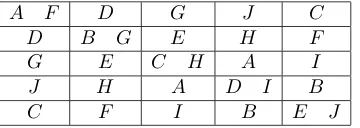
Example 8.3 The design in Figure 12 is taken from [157], rearranged to show the partitionsR andC as rows and columns. Here R∧C is not uniform, because some parts ofR∧Chave size one and others have size two. Moreover,Ris not orthogonal toC, becauseNRC =I5+J5when the rows

and columns are labelled in the obvious way. However,NRLNLC = 3NRC,

A F D G J C

D B G E H F

G E C H A I

J H A D I B

C F I B E J

Figure 12: A design for 30 units, with partitions into rows, columns and letters

8.2 Link with subspaces

Some observations from Section 7 are gathered here.

Proposition 8.4 LetR,CandLbe partitions ofΩ. Put QF =PF−PU

forF in{R, C, L}. IfR∨C=L∨R=L∨C=U then the following hold.

(i) VLR⊥VLC if and only ifQRQLQC= 0.

(ii) If VLR ⊥VLC thendim(VLR) + dim(VLC)≤nL−1.

(iii) IfR_IL,C_ILandVLR⊥VLC then nR+nC−1≤nL.

(iv) VR`L⊥VC`L if and only ifQR(Ie−QL)QC = 0.

(v) If R⊥C then QRQC = 0 and therefore VLR ⊥ VLC if and only if

VR`L⊥VC`L.

This shows that an alternative characterization of R and C having adjusted orthogonality with respect toL is that the subspacesVR`L and

VC`L are orthogonal to each other. Moreover, if, in addition,R⊥C, then

the subspacesVLR andVLC are orthogonal to each other. Then part (iii)

gives the following result.

Theorem 8.5 If R⊥C, R _I L, C _I L, and R and C have adjusted

orthogonality with respect toLthennR+nC−1≤nL.

8.3 A little history

Preece spent the year 1974–1975 in Australia: see [29]. At the end of his stay, he presented work on these designs at the Australian Conference on Combinatorial Mathematics in Adelaide: see [151]. This led Sterling and Wormald to give some constructions for such designs in [201] and Seberry and Street to take the ideas further in [187, 203].

Meanwhile, Eccleston and Russell had independently invented the idea of adjusted orthogonality, which they wrote asR(L)⊥C(L) in [72], where they proved Lemma 8.1. They introduced the name ‘adjusted orthogonal-ity’ in [73]. Papers [12, 19, 68, 69, 70, 74, 102, 184, 189, 190] followed, and the book [191] also had a section on adjusted orthogonality, but none of these mentioned the work of Preece.

Preece, Eccleston and Russell were all working in Statistics at univer-sities in Sydney during the last four months of 1974. They met for discus-sions during this time, and Preece was external examiner for Russell’s 1977 PhD thesis [183], whose Chapter 4 was devoted to adjusted orthogonality. Eccleston and Russell both report on Preece’s very thorough reading of this1_{. Nonetheless, when Preece cited [72] in his 1977 paper [154] it was}

only to say that this concept of orthogonality was not related to anyone else’s. However, his article [157] for the Genstat Newsletter did use the phrase ‘adjusted orthogonality’, and explained it very clearly in the con-text of Example 8.3. I have not found an instance of his using the phrase ‘adjusted orthogonality’ in the mainstream literature before [164].

Bagchi listed authors who had constructed designs with adjusted or-thogonality in [17], again with no mention of the many designs given by Preece in [147], and proved Theorem 8.5 in [18].

Eccleston and McGilchrist extended the ideas of [100] to three sub-spaces in [71] and applied their results to row–column designs. In particu-lar, they proved that the average variance of estimators of differences like

τi−τj is bounded below by a known function of the average variances in

the two block designs obtained when one of the partitions into rows and columns is ignored, and that this bound is achieved if rows and columns have adjusted orthogonality with respect to letters. Bagchi and Shah gen-eralized this to a stronger notion of optimality in [21], but with no mention of [71].

Independently of Eccleston, Russell, and their co-authors, but building on the work of Preece in [145, 147, 151], Morgan and Uddin in [123] defined a block design for two non-interacting treatment factors F and G to be anorthogonal BIBD ifF _BB,G_BB and kBNF G=NF BNBG; this last

condition is precisely adjusted orthogonality. The terminology OBIBD is also used in [1, 85, 120]; the first two of these state that the third condition

is the same as adjusted orthogonality. Rees presented [1] at the British Combinatorial Conference in Sussex (2001).

8.4 Adjusting for more than one partition

In [72], Eccleston and Russell proposed a more general version of ad-justed orthogonality. IfL is a set of partitions of Ω, putVL =PL∈LVL,

and letPL be the matrix of orthogonal projection ontoVL. By conven-tion,P∅=P{U}=PU =e−1Jee. In the notation of [72],R(L)⊥C(L) if

(V_R+V_L)∩V_L⊥ is orthogonal to (V_C+V_L)∩V_L⊥; equivalently,

XR>(Ie−PL)XC = 0.

In words,R andC have adjusted orthogonality with respect toL. In an important special case of this, F is a Tjur block structure and L=F \ {E}. ThenR andChave adjusted orthogonality with respect to Lif and only if the projections of VR and VC ontoWE are orthogonal to

each other, whereWE is the subspace defined in Section 4.3.

9

Adjusted balance

9.1 Terminology

Section 8 discussed adjusted orthogonality, which is a possible relation between partitionsF andGwhen everything is projected onto the orthog-onal complementV_H⊥ of VH for some other partitionH. What happens

whenF =G? In this case, for clarity, we writeF =G=LandH =B. Recall from Section 2 thatX_L>X_L is a diagonal matrix whose diagonal entries are the sizes of the parts ofL. ThusLis unform if and only ifX_L>X_L

is completely symmetric. Some authors say thatLis balanced. Following on from Section 8, it would be natural to say thatLhas adjusted balance with respect to B if X_L>(I_e−P_B)X_L is completely symmetric. This is always true whennL≤2, because thenL×nL matrixXL>(Ie−PB)XLis

symmetric and has zero row-sums.

The requirement thatX_L>(I_e−P_B)X_Lbe completely symmetric is the main part of the definition of balance in Section 5.3. For consistency with Section 5, I shall continue to say ‘is balanced with respect to’ rather than ‘has adjusted balance with respect to’, but this discussion does show that the ideas in Sections 5 and 8 are closely related. However, there is one twist. In Section 5, we required X_L>(Ie−PB)XL to be completely

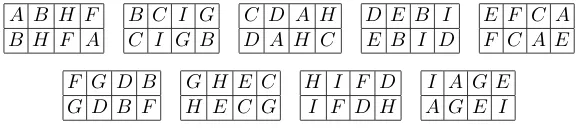
A B H F B H F A

B C I G C I G B

C D A H D A H C

D E B I E B I D

E F C A F C A E

F G D B G D B F

G H E C H E C G

H I F D I F D H

I A G E A G E I

Figure 13: Design in Example 9.1: there are nine letters in nine blocks, each of which is a 2×4 rectangle

This twist shows a difference between orthogonality and balance. If

F ₄Gthen F ⊥G, so we regard refinement as a special case of orthog-onality. However, ifF ₄G then X_F>(I_e−P_G)X_F = 0, so that F is not balanced with respect toG, as noted in Section 5.2.

9.2 General definition

We can now define balance with respect to a set of partitions in a way that is analogous to the more general definition of adjusted orthogonality in Section 8.4.

Definition Let G be a set of partitions of Ω, and let L be a partition of Ω. ThenLis balanced with respect toGifX_L>(I_e−P_G)X_Lis completely symmetric but not zero.

It is immediate thatLcannot be balanced with respect toGif there is anyGin Gfor whichG₄L. As in Section 8.4, an important special case occurs whenG=F \ {E} for some Tjur block structureF. In this case,

Lis balanced with respect toG if it is balanced with respect toGfor all in G andX_L>(I_e−P_G)X_L is not zero. The following example shows that it is possible to achieve balance with respect toG without having balance with respect to allGinG.

Example 9.1 The design in Figure 13 has 72 units, in nine blocks, each of which is a 2×4 rectangle. Nine letters have been allocated to the units. Denote byB, R, C and L the partitions into blocks, rows, columns and letters respectively. ThenPR,C,B=PR+PC−PB and so

XL>(Ie−PR,C,B)XL=XL>(Ie−PC)XL−XL>(PR−PB)XL.

In this design, the two rows in each block have exactly the same set of letters, with the result that X>

D E F G H I

H I G C A B

C A B E F D

B H E I C F

F C I D G A

G D A B E H

Figure 14: Row–column design in which letters are balanced with respect to{R, C}while rows and columns have adjusted orthogonality with respect to letters

X_L>(I_e−P_R,C,B)X_L = X_L>(I_e−P_C)X_L, which is completely symmet-ric and nonzero, because L _B C. Hence L is balanced with respect to {R, C, B}, even though it is not balanced with respect to either R or B. In fact, in this examplePR,C,B =PR,C because R≺B, and soL is also

balanced with respect to{R, C}.

9.3 Balance with respect to a pair of partitions

The most common use of this more general concept of balance is for the case that G ={R, C} and R∨C = U, so that we are interested in the projection of the data onto (VR+VC)⊥. Let QRC be the matrix of

orthogonal projection onto (V_R+V_C)∩V_U⊥; and putQR=PR−PU and

QC =PC−PU. Then L is balanced with respect to the pair {R, C} if

X_L>(I_e−Q_RC−P_U)X_L is completely symmetric but not zero.

This terminology is consistent with that in [25], but it is not ideal, because ‘Lis balanced with respect toR andC’ might mean ‘L_IRand

L_IC’ or it might mean ‘L is balanced with respect to{R, C}’. In [151], Preece calls it ‘Lhas overall total balance with respect to the rest of the design’; in later papers this becomes ‘Lis fully balanced . . . ’.

IfR_IC then equation (7.1) givesX_L>Q_RCX_L. If, additionally, either

L⊥R or L⊥C then X>

LQRCXL is a scalar multiple of one of XL>QRXL

andX>

LQCXL, so the properties of XL>QRCXL follow from those of the

binary relations betweenLandR and betweenL andC.

If R⊥C then QRC =QR+QC and so the properties ofXL>QRCXL

are derivable from those ofX_L>Q_RX_LandX_L>Q_CX_Lconsidered together. It may be possible for their sum to be completely symmetric even though neither is. For example, in a resolvable BIBD in whichnB = 2kB it may

be possible to allocate the letters to the cells of akB×kB square in such

(the blocks are the complements of those in Figure 1). In this design, it is also true that rows and columns have adjusted orthogonality with respect to letters. Many more examples are given in [113, 134]. Preece found 345 species (that is, merging isomorphism classes obtainable from each other by interchanging rows and columns) of designs with these parameters and properties in [149, 153], while McSorley and Phillips completed the enumeration to 348 by a computer search reported in [117].

9.4 Three-way balance with pairwise balance

Suppose that C _IR. Equation (7.1) shows that the condition forL

to be balanced with respect to{R, C} is that the matrix

(1−λ)XL>XL−(1−λ)XL>PUXL−(1−λ)XL>QRXL−XL>QCXL

+X_L>Q_RQ_CX_L+X_L>Q_CQ_RX_L−X_L>QRQCQRXL

is completely symmetric but not zero. IfL_IR andL_ICthen the first four terms are completely symmetric, and so the first part of this condition becomes

kR(NLRNRCNCL+NLCNCRNRL)−NLRNRCNCRNRL

is completely symmetric. (9.1)

Condition (9.1) is given explicitly in [151].

If, in addition, C and L have adjusted orthogonality with respect to

R, then Lemma 8.1 shows that NCRNRL is a scalar multiple of NCL.

Therefore the matrix in (9.1) is a multiple ofNLCNCL, which is completely

symmetric because L _I C. Thus adjusted orthogonality gives a special case of this type of three-way balance.

In [147], Preece gave 59 designs with three partitions R, C and L

satisfying nR = nC < nL, R B L, C B L, R ./ C and NRLNLC =

kLNRC. It follows thatRandC have adjusted orthogonality with respect

to letters, thatRis balanced with respect to{C, L}, and thatCis balanced with respect to{R, L}. Figure 15 shows an example. Street generalized his constructions in [203] to give infinite families of designs, and widened the scope by relaxing the final condition to allow NRLNLC to be any

completely symmetric matrix. Agrawal and Sharma gave further designs of this type in [10].

On the other hand, if nL ≤ nC = nR then equation (7.2) gives the

following (ignoring the possibility thatX_L>(Ie−QRC−PU)XL might be

L I F J G D A

E M J G K A B

B F N K A L C

M C G H L B D

C N D A I M E

N D H E B J F

K H E I F C G

H I J K L M N

Figure 15: A design for 56 units, with partitions into rows, columns and letters: blank cells indicate empty row-column intersections

Proposition 9.2 Suppose that R ./ C, L _IR and L _I C. Then L is balanced with respect to{R, C} if and only if

NLRNRCNCL+NLCNCRNRL is completely symmetric. (9.2)

A stronger condition is

NLRNRC is a linear combination ofNLC andJnLnC. (9.3)

Proofs of the following are in [25].

Proposition 9.3 If R ./ C,L_IR andL_IC then the following hold.

(i) Condition (9.3) implies condition (9.2).

(ii) If nL = nC and condition (9.2) is satisfied for the ordered triple

(L, R, C)then it is satisfied for any permutation of{L, R, C}.

(iii) If nL = nC and condition (9.3) is satisfied for the ordered triple

(L, R, C)then it is satisfied for any permutation of{L, R, C}.

A B C D

E A B F

D A F G

C E A G

B G D E

F C G B

E F D C

A E B C

B F C D

C G D E

F D A E

G E B F

G A F C

D A B G

(a) (b)

Figure 16: Two designs for 28 units, with partitions into rows, columns and letters: blank cells indicate empty row-column intersections

10

Three partitions

10.1 Supreme sets of uniform partitions

For simplicity, from now on we confine our interest to uniform parti-tions on Ω. The following definition is taken from [32].

Definition A set F of partitions on Ω issupreme if F ∪ {U} is closed under taking suprema.

We shall examine supreme setsFof uniform non-trivial partitions of Ω with the property that ifF andGare inFthen at least one of the following holds: (i)F is orthogonal toG(this includesF ≺GandG≺F); (ii) at least one ofF andGis strictly balanced with respect to the other.

Pearce and co-authors discussed sets of (usually) uniform partitions in [98, 134] and introduced notation for various binary relations between them. Preece augmented the notation in [145] and displayed the relations in a matrix whose rows and columns are labelled by the partitions. The diagonal is empty. IfF 6=Gthen the (F, G)-entry is O (for ‘orthogonal’) ifF is strictly orthogonal to Gand F ∧Gis uniform; it is T (for ‘total balance’) ifF is binary balanced with respect toGbut not orthogonal to

G; it isT0 _{(with the connotation that the transpose indicates the reverse} relationship) ifF is neither orthogonal nor binary balanced with respect toGbutGis binary balanced with respect toF.

row–column designs are

R C L R

C L





− O O O − T O T −





and

R C L R

C L





− O T

O − T T0 T0 −





respectively.

In [32], Bailey and Cameron convey the same information by showing each partition as a vertex of a directed graph and labelling the edges with symbols to show the relationships. Here we shall simply use the symbols ⊥,⊥,≺,,_C,_Band./.

10.2 Two partitions

Suppose that F ={F, G}, where F and G are distinct uniform non-trivial partitions. IfF is supreme, then, up to renaming, eitherF ≺Gor

F∨G=U. The first case gives a poset block structure withP ={1,2,3} and 3<2<1, whereF =F_{1,2} andG=F{1}.

If F ∨G = U and F ⊥ G then F⊥G and all parts of F ∧G have the same size, by Proposition 4.1. ThenF andGcan be regarded as the partitions of a rectangle into rows and columns, with each row-column intersection containing the same number of units. IfF∧G=E this is the poset block structure defined byP ={1,2}with trivial partial order.

If F ∨G = U but F is not orthogonal to G then, up to renaming,

F _BG. Altogether, we have these possible structures.

A.1 The poset block structure defined by P ={1,2,3} and 3 <2 <1, withF={F_{1}, F{1,2}}.

A.2 The poset block structure defined byP ={1,2}with trivial partial order, withF ={F{1}, F{2}}.

A.3 The poset block structure defined byP ={1,2,3}, 3<1 and 3<2, withF={F{1}, F{2}}.

A.4 F _BGbut Gis not balanced with respect to F, so thatnF < nG.

A.5 F ./ G, so thatnF =nG.

10.3 Three partitions: three orthogonal relations

G≺H orF ∨G=H. The first case gives a poset block structure with P = {1,2,3,4} and 4 < 3 < 2 < 1, where F = F{1,2,3}, G = F{1,2} and H = F{1}. In the second case, the parts of H can be considered as rectangles, each of which is partitioned into rows and columns as in structures A.2 or A.3: the first of these gives Example 4.4. BecauseF, G

andH are all uniform, Proposition 4.1 shows thatF∧Gis uniform. If only one supremum isU, suppose that it isG∨H. ThenF≺Gand

F ≺H, soF ₄G∧H. This gives two cases: F=G∧H andF≺G∧H. If precisely two suprema areU, suppose that they areF∨H andG∨H. Then either F ≺ G or G ≺ F, and we obtain a poset block structure like the one in Example 4.5. If all three suprema areU then we have an orthogonal array of strength two. This is not necessarily derived from a poset block structure: for example, F, G and H could be three of the partitions in Figure 7.

This gives the following possible structures.

B.1 The poset block structure defined by P ={1,2,3,4} and 4 < 3 < 2<1, withF={F{1}, F{1,2}, F{1,2,3}}.

B.2 The poset block structure defined byP ={1,2,3}, 2<1 and 3<1, withF={F{1}, F{1,2}, F{1,3}}.

B.3 The poset block structure defined by P={1,2,3,4}, 4<3<1 and 4<2<1, withF ={F_{1}, F{1,2}, F{1,3}}.

B.4 The poset block structure defined byP ={1,2,3}, 3<1 and 3<2, withF={F{1}, F{2}, F{1,2}}.

B.5 The poset block structure defined by P={1,2,3,4}, 4<3<1 and 4<3<2, withF ={F{1}, F{2}, F{1,2,3}}.

B.6 The poset block structure defined by P ={1,2,3} and 2<1, with F={F{1}, F{1,2}, F{3}}.

B.7 An orthogonal array of strength two containing three partitions.

10.4 Three partitions: two relations of orthogonality and one of balance

Suppose thatF ={F, G, H}, whereF, GandH are distinct uniform non-trivial partitions,F is supreme, F _BG, F ⊥H andG ⊥H. Since

F∨G=U, we cannot haveH F andH G, because that implies that

H_<F∨G.