The Time Optimal Problems for Controlled Fuzzy R Solutions

doi:10.4236/ica.2011.22018 Published Online May 2011 (http://www.SciRP.org/journal/ica)

The Time-Optimal Problems for Controlled Fuzzy

R-Solutions

Andrej V. Plotnikov, Tatyana A. Komleva, Irina V. Molchanyuk

Odessa State Academy of Civil Engineering and Architecture, Odessa, Ukraine E-mail: [email protected], [email protected], [email protected]

Received April 21, 2011; revised May 12, 2011; accepted May 15, 2011

Abstract

In the present paper, we show the some properties of the fuzzy R-solution of the control linear fuzzy differ-ential inclusions and research the time-optimal problems for it.

Keywords:Fuzzy Differential Inclusions, Control Problems, Time-Optimal Problems, Fuzzy R-Solution

1. Introduction

The first research of the differential equations with set- valued right-hand side has been fulfilled by A. Marchaud [1,2] and S. C. Zaremba [3]. In the early sixties, T. Wazewski [4,5], A. F. Filippov [6] had been obtained fundamental results about existence and properties of solutions of the differential equations with set-valued right-hand side (differential inclusions). Connection de-riving between differential inclusions and optimum con-trol problems was one of the most important outcomes of these papers. These outcomes became impulse for de-velopment of the theory of differential inclusions [7-9].

Considering of the differential inclusions required to study properties of set-valued maps, i.e. an elaboration the whole tool of mathematical analysis for set-valued maps [7,10,11].

In work [12] annotate of an R-solution for differential inclusion is introduced as an absolutely continuous set- valued maps. Various problems for the R-solution theory were considered in [8,13]. The basic idea for a develop-ment of an equation for R-solutions (integral funnels) is contained in [14].

In the eighties the last century the control theory in the conditions of uncertainty began to be formed. The con-trol differential equations with set of initial conditions [15-17], control set differential equations [18-21] and the control differential inclusions [21-32] are used in the given theory for exposition of dynamic processes.

In recent years, the fuzzy set theory introduced by Zadeh [33] has emerged as an interesting and fascinating branch of pure and applied sciences. The applications of fuzzy set theory can be found in many branches of

re-gional, physical, mathematical, differential equations, and engineering sciences. Recently there have been new advances in the theory of fuzzy differential equations [34-47] and inclusions [48-53] as well as in the theory of control fuzzy differential equations [54-57] and inclu-sions [57-59].

In this article we consider the some properties of the fuzzy R-solution of the control linear fuzzy differential inclusions and research the time-optimal problems for it.

2. The Fundamental Definitions and

Designations

Let comp R

 

n



conv R

 

n



be a set of all nonempty (convex) compact subsets from the space Rn,







 

 



0

, min _r , _r

r

h A B S A B S B A



  

be Hausdorff distance between sets A and B, S_r

 

A

is r-neighborhood of set A.

Let _En be the set of all _{u R:} n_

 

_0,1

such that u satisfies the following conditions:

1) u is normal, that is, there exists an 0

n

x R such that u x

 

0 1;

2) u is fuzzy convex, that is,







1



min



   

,



u x  y  u x u y

n

for any x y, R and 0  1; 3) u is upper semicontinuous, 4)

 

u 0 cl x



Rn:u x

 

0



n

 is compact. If , then is called a fuzzy number, and is said to be a fuzzy number space. For

uE u _En

 

_u  



_x_Rn:_{u x}

 





.

Then from (1) - (4), it follows that the -level set for all 0 1

 

_u _{conv R}

 

n  

.

Let  be the fuzzy mapping defined by 

 

x 0 if and .

0

x 

 

0 1

: n n

D E E

Define  







by the relation

 

0,

   





0 1

, sup ,

D u v h u  v



 

 ,

where h is the Hausdorff metric defined in _{comp R}

 

n

. Then D is a metric in _En.

Further we know that [60]:

1)



_En,_D is a complete metric space,



D u w





2)  ,vw



D u v



, for all ,





, ,

n

u v wE 3) D  u, v   D u v

 

, for all , n and

u vE R

  .

Definition 1. [36] A mapping : 0,

 

n

F T E is measurable if for all  

 

0,1 the set-valued map

 



: 0, n



F_ T conv R defined by F_

 

t  F t

 

 is Lebesgue measurable.

Definition 2. [36] A mapping : 0,

 

n

F T E is said to be integrably bounded if there is an integrable function

such that

 

h t x t

 

h t

 

for every x t

 

F0

 

t .

Definition 3. [36] The integral of a fuzzy mapping

 

: 0, n

F T E

T T

is defined levelwise by

 

 

0 0

d d

F t t  F_ t t

  









 

. The set

 

0

d

T

F_ t t



of all

 

0 d

T

f t t



such that : 0,

 

n

f T R is a measurable selection for F_: 0,

 

T conv R

 

n for all 

 

0,1.

Definition 4. [36] A measurable and integrably bounded mapping F: 0,

 

T En is said to be integra- ble over

 

0,T if

 

0

d n

T

F t tE



.

Note that if F: 0,

 

T En is measurable and inte-grably bounded, then F is integrable. Further if

 

: 0, n

F T E is continuous, then it is integrable. Now we consider following control differential equa-tions with the fuzzy parameter



, , ,

  

, 0 0,

x f t x w v x x (1) where x means d

d x

t ; tR is the time;

n

xR

k

is the state; is the control; is the fuzzy parameter;

m

wR v V E

k n

: n m

f RR R 

 

m

onv R

R R .

Let be the measurable set-va- lued map.

: 

W R c

Definition 5. The set of all measurable single- valued branches of the set-valued map is the set of the admissible controls.

LW

 

W 

Further we consider following control fuzzy

differen-tial inclusions



, ,

  

, 0 0, xF t x w x x

n

(2) where F R: RnRm E is the fuzzy map such that F t x w



, ,



 f t x w V



, , ,



.

Obviously, the control fuzzy differential inclusion (2) turns into the ordinary fuzzy differential inclusion

   

, , 0 0,

x  t x x x (3) if the control w

 

 LW is fixed and

 

t x, F



t x w t, ,

 



  .

If right-hand side of the fuzzy differential inclusion (3) satisfies some conditions (for example look [12]) then the fuzzy differential inclusions (3) has the fuzzy R-so- lution.

Let X t

 

denotes the fuzzy R-solution of the differ-ential inclusion (3), then X t w



,



denotes the fuzzy R-solution of the control differential inclusion (2) for the fixed w

 

 LW.

Definition 6. The set Y T

 





X



T w,

  

:w  LW



be called the attainable set of the fuzzy system (2).

3. The Some Properties of the Fuzzy

R-Solution

Further in the given paper, we consider following control linear fuzzy differential inclusions

 

   

, , 0 0,

xA t x G t w x x (4) where A t

 

is



n n



dimensional matrix-valued function; G R: _Rm _En is the fuzzy map.



In this section, we consider the some properties of the fuzzy R-solution of the control fuzzy differential inclu-sion (4).

Let the following condition is true. Condition A:

A1. A

 

 is measurable on

 

0,T ;

A2. The norm A t

 

of the matrix A t

 

is inte-grable on

 

0,T ;

A3. The set-valued map :



₀,



 

m

W t T conv R is measurable on

 

0,T ;

A4. The fuzzy map : 0,

 

m n

G T R E satisfies the conditions

1) measurable in t; 2) continuous in w;

A5. There exist v

 

 L2

 

0,T and l

 

 L2

 

0,T

such that

 



, 0



 

, ,



 

,



 

h W t v t D G t w  l t almost everywhere on

 

0,T and all w W t

 

.

A6. The set Q t

 







, ( ) :w t

  

w  LW





G t  is

com-pact and convex for almost every t 0,T



, i.e.

 

 

n

Q t conv E .

Then for every there exists the fuzzy R-solution

 

w  LW





,

X w such that 1) the fuzzy map X

 

,w has form

 

 

 

1

 



 



0

0

, ,

t

d X t w   t x   t



 s G s w s s, where t

 

0,T ; is Cauchy matrix of the differ-ential equation

 

t



 

xA t

n x  E w t X(, )

;

1) for every t

 

0,T ;

2) the fuzzy map X

 

,w is the absolutely continuous fuzzy map on

 

0,T .

Proof. 1. Show that X t w



,



is the fuzzy R-solution of the fuzzy system (4). We have

 

 

 

 



 



 

 

 



 



 

 

 

 

1 0 0 1 0 0 1 0 0 , , d

( , d

t

t

t

, d

X t w t x t s G s w s s

t x t s G s w s s

t x t s G s w s s

                 _      _ _  _        _ _







    

for all 

 

0,1



w

, t0 and w

 

 LW. Since



,

X t 

 

  is the R-solution of the control differential inclusion

 

( ,

 

,

 

0 0

xA t x_G t w t _ x t x

(see [30]), we obtain that X t w

 

, is fuzzy R-solution of the control fuzzy differential inclusion (4).

2. By [36] and Condition A we have that

 

, n

X t w E for all t0 and w

 

 LW.

 

,

X t w

3. From [30] we have that _ _ is the abso-lutely continuous set-valued map on

 

0,T for all

 

0,1

 , i.e. X t w



,



is the absolutely continuous fuzzy map on

 

0,T . The theorem is proved.

Theorem 2.Let the condition A is true.

Then the attainable set Y T

 

is compact and convex. Proof. It is easy to check that

 

 

 

1

   

0

0

d

T

Y T   T x   T



 s Q s s

and

 

 

 

1

   

0 0

d

T

Y T    T x   T  s Q s  s

   

 



  ,

where _Q t

 

_: 0,

 

T conv conv R



 

n



for all

 

0,1



T

. From [20,21,30,57] we obtain that

 

1

   



 

0

d n

T  s Q s  s conv conv R

  _ _ 





for all

 

0,1

 , i.e. Y T

 

conv E

 

n . This ends the proof. We obtained the basic properties of the fuzzy R-solu-

tion of systems (4). Now, we consider the some fuzzy control problems.

4. Time-Optimal Problems

Consider the following time-optimal problem: it is nec-essary to find the minimal time T and the control

 

*

w  LW such that the fuzzy R-solution of system (4) satisfies one of the conditions:



*



, k

X T w S  , (5)



*



, k

X T w S , (6)



*



, k

X T w S , (7) where SkEn is the fuzzy terminal set.

It is obvious that optimum time and optimum controls for these problems will be different.

Theorem 3. (necessary optimal condition for the time-optimal problem (4), (5)). Let the condition A is true and the pair



*

 



,

T w  is optimality of the control problem (4), (5).

Then there exists the vector-function , which is the solution of the system

 

 

 

, 0

 

1



T

A t T S

     



such that

1)

 

 

 



 

 



1 1

*

, , max , ,

w W t

C G t w  t C G t w  t



_{ } _{  }

_{ }   

 

almost everywhere on

 

0,T ;

2)





 



 

 



,

1 ₁

*

, , k ,

C_X T w _  T  C S  T

 

where



,



max



1 1



, , n n n

p P

C P p p  R



   

 

n

Pconv R . Proof. Let *

 

w  is the optimal control and

 

* , X w is the optimal fuzzy R-solution of the problem (4), (5), i.e.

1) X T w



, *



Y T

 

; 2)



*



, k .

X T w S   From 1) and 2) we have

 1







 

1

max , k ,

X Y T

C X  C S 



_ _    (8)

for all  S1

 

0 .

Consequently

 1 ₁ 







 



1 0

max min , k , 0.

S X Y T

p C X C S

   _ _    1  0 

From _X T w



, *



_ 

 

S_k 1   we have 1

*

 











 

1



, , , _k ,

q T C_X T w _ C S 

for all

From 1 we have that the function

 

1 0 S  . Theorem an



,



q T

ve is continuous on RS1

 

0 .

If q T



,



0 for all S1

 

0 then we ha

 

_{ }



0

0

min 0

S

q T q T

 





 . Hence there exists

1

,   T

su equently

0



for all i.e.

It contradicts that is optimal time.



ch that q0

 

 0. Cons we have





1



 

₁



*

, , ,

C__X  w  _C S 

  _ k

 

1 0 S

 ,



_, *



1

 

1

k

X  w S

  _{ }

   .

T

If, p0

   







 



1 10 1 , , ,

X Y T

k

C X

C X C S









 

1

max min , _k

S  C S 

   _ _      1  

and _X T w



, *



 _ X

ce there exists 

, than we have a contradiction. Hen S1

 

0 such that



*



,w ,

 1





1

max , ,

X Y T

C X T  C X 

_ _   _{ }        





1



 

₁



*

, , _k ,

C_X T w _ _ C S  .

  

Consequently

 

0

C T

 



 



 

 

 



 



1 1 * 1 1 0

, d ,

max , d ,

T

T w LW

s G s w s s

C T s G s w s s

       _{ }    _{ }      _{ }  



    

Then we have

   





 

 



 



 



 

  





1 1 * 1 1 , ,

max , ,

w W t

C T s G s w s

C T s G s w

     _{   }   _{ }     _ _    

for almost every s

 

0,T . If

 



 

 



 

 





1 1 T T T t t T t            , than the theorem 3 is proved.

Theorem 4. (necessary optimal condition for the tim .Let the condition A is tr

system



e-optimal problem (4), (6))

 



*



ue and the pair T w,  is optimality of the control problem (4), (6).

Then there exist the vector-function 

 

 , which is the solution of the

 

, 0

 

 

1

 

T

A t T S

    

d  

 

0,1 such that 1)

 

*

 



 

 



( )

, , max , ,

w W t

C G t w   t C G t w   t



_{ } _{ }

_{ }  _{ }

  

almost everywhere on

 

0,T ; all

2) for  

 

0,1



*



 



 

 



, , _k ,

C_X T w _  T C S   T

 

and



*



 



 

 



, , _k ,

C_X T w _  T C S   T

  .

This changes

theorem is proved analogous theorem 5 with little of condition (8):

for all  

 

0,1

 







 



max , _k , 0

X Y T

C X C S



_ _

  

 

for all  S1

 

0 and there exist  

 

0,1 and

n

R

 such that

 







 



max , _k , 0

X Y T

C X C S





 

_ _   .

Theorem 5. (necessary optimal condition for the time-optimal problem (4), (7)). Let the condition A is true and the pair



T w, *

 





is optimality of the control problem (4), (7).

Then there exist the vector-function 

 

 , which is the solution of the system

 

,

T

A t

 

T S1

 

0

     

and  

 

0,1 such that 1)

 

*

 





 



( )

, , max , ,

w W t

C G t w   t C G t w   t



_{ } _{  }

_{ }  _{ }

 



almost everywhere on

 

0,T ; all

2) for  

 

0,1



_, *



_,

 



 

_,

 



k

C__X T w _  T _C S   T and



*



 



 

 



, , _k ,

C_X T w _  T C S   T

  .

Also little ch

this theorem is proved analogous theorem 5 with anges of condition (8):

for all  

 

0,1

 





 

k

X Y T

C X C S



_ _







 ,

max , , 0

for all  S1

 

0 and there exist  

 

0,1 and

n

 







 



max , _k , 0

X Y T

C X C S





 

_ _

  .

Example. Consider the following control linear fuzzy differential inclusions

 

, 0 0,

x  x w F x  (9) where

x is the state; w W  



1,1



is the control;

1

FE is the fuzzy set, where



 

0, 0, 5

2 1, 0, 5

3, 1 1

1, 5

f

f

f

f 

  _{ } 



   

1

f 

2 , 5

0,

f

f

  

.

Consider the following time-optimal problem: it is necessary to find the minimal time an the control

W such that the fuzzy R-s ion f system (9) satisfies of the condition (5), where t e fuzzy terminal

such, that

T

olut h

d o

 

*

w  L

set SkE1

 

0, 1, 75

4 7, 1, 75 2

1, 2 3

4

x

x x

x x

x 13, 3 x 3, 25

0, 3, 25 x



 

 _{  } 

_       . 

 

The control and time will be optimum pair fo e given pr set

 

* ₁

w t 

r th

 

ln 2

T 

oblem. Fuzzy



*



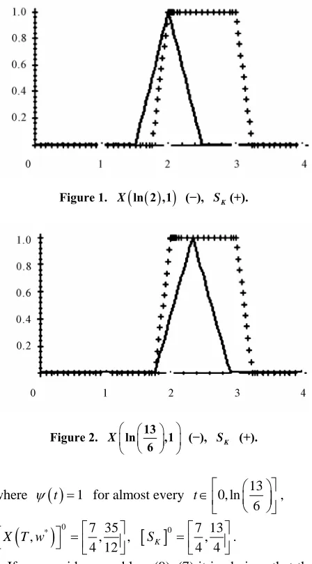
[image:5.595.313.537.78.483.2]

, X T w Figure 1.

inal set are shown in Obviously, this optimal pair satisfies to conditions of th

and fuzzy term SK

e theorem 3:

1)



w t*

   

, t



C W



,

 

t



for almost every

 

0, ln 2

t _ _;

2)





 

for almost every



e consider the time-optimal problem (9), (6 hen

 

 





1 ₁

*

, , _k ,

C_X T w _  T _ C S  T

  ,

where 

 

t 1 t _0, ln 2

 

_,





1

*

X T w,  2

   ,.

  

SK 1 2, 3

If w ) t

the control w t*

 

1 and time ln 13 6

T   

  will op-

timum pair. Fuzzy set

be



_, *



X T w and fuzzy terminal set

K

S

co

are shown in Figure 2. This optimal pair satisfies to nditions of the theorem 4:

1)



w t*



  

, t



C W



,

 

t



for almost every 13

0, ln 6 t_ _ __

 

 ;

2) C _X T w



, *



 _0, 



T



 C



 

S_k 0,

 

T

  ,

 



ln 2 ,1



X (−), SK

Figure 1. (+).

   

 _ _ 

 

13

ln ,1

6

[image:5.595.108.239.324.395.2]

X (−), S_K

Figure 2. (+).

where for almost every 0, ln 13 6 t_ _ __

 

 

 

t 1

  ,





0

* 7 35

, , ,





4

 

0 7 13

12

X T w  

 _{   }

  _{ } _4, _. 4

K

S  

If we consider a problem (9), (7) it is obvious that the olution does not exist.

5. Conclusions

In the last decades, a nu ber of works de ted to prob-le

works fall into a subdivision of theory, namely, the theory of process

tainty and fuzzy conditions. This is s

m vo

ms of optimal control of set-valued trajectories (fuzzy trajectories, trajectory bundles or an ensemble of

trajec-ories) appeared; these t

the optimal control ontrol under uncer c

to describe behavior of objects. The rea-so

the necessary conditions of opti-m

. Marchaud, “Sur les Champs de Demicones et

Equa-erentilles du Premier Ordre,” Bulletin de tique de France, Vol. 63, 1934, pp

, No. 4, 1967, pp. equations that describe the behavior of the object are simplified and one should estimate the consequences of such a simplification. Therefore, if is possible to divide the articles devoted to this direction into two types char-acterized by the following distinctive features:

1) there exists an incomplete or fuzzy information on the initial data;

2) the equations describing the behavior of the object to be controlled are assumed to be inexact, for example, they can contain some parameters whose exact values and laws of variation are unknown but the domain of their values is fuzzy.

In the second case, fuzzy differential inclusions are frequently used

n is that, first this approach is most obvious and, sec-ond, theory of fuzzy and ordinary differential inclusions is well found and is rapidly developed at the present time.

In the present paper,

al of control for a system of the latter form of equations with the fuzzy R-solutions are formulated and proved.

6. References

[1] A

tions Differentielles du Premier Order,” Bulletin de la Société Mathématique de France, Vol. 62, 1934, pp. 1-38.

] A. Marchaund, “Sur les Champs des Deme-Droites et

[2 les

Equations Diff

Société Mathéma

la

. 1-38.

[3] S.C. Zaremba, “Sur une Extension de la Notion d’Equa- tion Differentielle,” Reports of the Paris Academy of Sciences, Vol. 199, 1934, pp. 1278-1280.

[4] T. Wazewski, “Systemes de Commande et Equations au Contingent,” Bulletin de l’Academie Polonaise des Sciences. Serie des Sciences Mathematiques, Astronomiques et Physiques, No. 9, 1961, pp. 151-155.

[5] T. Wazewski, “Sur une Condition Equivalente e L’Equation au Contingent,” Bulletin de l’Academie Polonaise des Sci-ences. Serie des Sciences Mathematiques, Astronomiques et Physiques, No. 9, 1961, pp. 865-867.

[6] A. F. Filippov, “Classical Solutions of Differential Equa- tions with Multi-Valued Right-Hand Side,” SIAM Journal on Control and Optimization, Vol. 5

609-621. doi:10.1137/0305040

[7] J.-P. Aubin and A. Cellina, “Differential Inclusions. Set-Valued Maps and Viability Theory.” Springer-Verlag, Berlin-Heidelberg-New York-Tokyo, 1984.

the Theory of Differen-tial Inclusions,” Graduate Studies in Mathematics, Vol.

6.

[8] V. A. Plotnikov, A. V. Plotnikov and A. N. Vityuk, “Dif- ferential Equations with Multivalued Right-Hand Sides,”

Asymptotics Methods, AstroPrint, Odessa, 1999. [9] G. V. Smirnov, “Introduction to

41, American Mathematical Society, Providence, 2002.

[10] J.-P. Aubin, “Mutational Equations in Metric Spaces,”

Set-Valued Analysis, Vol. 1, No. 1, 1993, pp. 3-4

doi:10.1007/BF01039289

[11] J.-P. Aubin and H. Frankovska, “Set-Valued Analysis,”

Birkhauser, Systems and Control: Fundations and Appli-

pike Systems,” Nauka i Tekhnika,

ntial Inclusion,” Matematicheskie Zametki,

rad University, Leningrad, 1980.

Stability of Motion. Lyapunov Methods

cations, 1990.

[12] A. I. Panasyuk, “Quasidifferential Equations in a Metric Space,” Differentsial’nye Uravneniya, Vol. 21, No. 8, 1985, pp. 1344-1353.

[13] A. I. Panasyuk and V. I. Panasyuk, “Asymptotic Turn Optimization of Control

Minsk, 1986.

[14] A. A. Tolstonogov, “On an Equation of an Integral Fun-nel of a Differe

Vol. 32, No. 6, 1982, pp. 841-852.

[15] D. A. Ovsyannikov, “Mathematical Methods for the Con- trol of Beams,” Lening

[16] V. I. Zubov, “Dynamics of Controlled Systems,” Vyssh Shkola, Moscow, 1982.

[17] V. I. Zubov, “

and Their Application,” Vyssh Shkola, Moscow, 1984.

[18] A. V. Arsirii and A. V. Plotnikov, “Systems of Control over Set-Valued Trajectories with Terminal Quality Cri- terion,” Ukrainian Mathematical Journal, Vol. 61, No. 8, 2009, pp. 1349-1356. doi:10.1007/s11253-010-0280-3

[19] N. D. Phu and T. T. Tung, “Some Results on Sheaf-So- lutions of Sheaf Set Control Problems,” Nonlinear Analy- sis, Vol. 67, No. 5, 2007, pp. 1309-1315.

doi:10.1016/j.na.2006.07.018

[20] A. V. Plotnikov, “Controlled Quasidifferential Equations and Some of Their Properties,” Differential Equations, Vol. 34, No. 10, 1998, pp. 1332-1336.

[21] V. A. Plotnikov and A. V. Plotnikov, “Multivalued Dif-

nt Conditions for Optima-

7/BF02366480

ferential Equations and Optimal Control,” Applications of Mathematics in Engineering and Economics,Heron Press, Sofia, 2001, pp. 60-67.

[22] G. N. Konstantinov, “Sufficie

lity of a Minimax Control Problem of an Ensemble of Trajectories,” Soviet Doklady Mathematics, Vol. 36, No. 3, 1988, pp. 460-463.

[23] S. Otakulov, “On the Approximation of the Time-Opti- mality Problem for Controlled Differential Inclusions,”

Cybernetics and Systems Analysis, Vol. 30, No. 3, 1994, pp. 458-462. doi:10.100

908040152

[24] S. Otakulov, “On a Difference Approximation of a Con- trol System with Delay,” Automation and Remote Control, Vol. 69, No. 4, 2008, pp. 690-699.

doi:10.1134/S0005117

ttainability Set of

Control of Pencils of [25] A. V. Plotnikov, “Linear Control Systems with Multi-

valued Trajectories,” Kibernetika, No. 4, 1987, pp. 130- 131.

[26] A. V. Plotnikov, “Compactness of the A

a Nonlinear Differential Inclusion that Contains a Con-trol,” Kibernetika, No. 6, 1990, pp. 116-118.

cal Journal, Vol. 33, Trajectories,” Siberian Mathemati

No. 2, 1992, pp. 351-354.doi:10.1007/BF00971112

[28] A. V. Plotnikov, “Two Control Problems under Uncer- tainty Conditions,” Cybernetics and Systems Analysis, Vol. 29, No. 4, 1993, pp. 567-573.

doi:10.1007/BF01125871

[29] A. V. Plotnikov, “Necessary Optimality Conditions for a Nonlinear Problems of Control of Trajectory Bundles,”

Cybernetics and Systems Analysis, Vol. 36, No. 5, 2000, pp. 729-733. doi:10.1023/A:1009432907531

[30] A. V. Plotnikov, “Linear Problems of Optimal Control of Multiple-Valued Trajectories,” Cybernetics and Systems Analysis, Vol. 38, No. 5, 2002, pp. 772-782.

doi:10.1023/A:1021899111846

[31] A. V. Plotnikov and T. A. Komleva, “Some Properties of Trajectory Bunches of a Controlled Bilinear Inclusion,”

Ukrainian Mathematical Journal, Vol. 56, No. 4, 2004, pp. 586-600. doi:10.1007/s11253-005-0114-x

[32] A. V. Plotnikov and L. I. Plotnikova, “Two Problems of Encounter under Conditions of Uncertainty,” Journal of Applied Mathematics and Mechanics, Vol. 55, No. 5, 1991, pp. 618-625.

doi:10.1016/0021-8928(91)90108-7

[33] L. A. Zadeh, “Fuzzy Sets,” Information and Control, No. 8, 1965, pp. 338-353.

doi:10.1016/S0019-9958(65)90241-X

[34] B. Bede and S. G. Gal, “Solutions of Fuzzy Differential Equations Based on Generalized Differentiability,”

Communications in Mathematical Analysis, Vol. 9, No. 2, 2010, pp. 22-41.

[35] M. H. Chen, D. H. Li and X. P. Xue, “Periodic Problems of First Order Uncertain Dynamical Systems,” Fuzzy Sets and Systems, Vol. 162, No. 1, 2011, pp. 67-78.

doi:10.1016/j.fss.2010.09.011

[36] O. Kaleva, “Fuzzy Differential Equations,” Fuzzy Sets and Systems, Vol. 24, No. 3, 1987, pp. 301-317.

doi:10.1016/0165-0114(87)90029-7

[37] O. Kaleva, “A Note on Fuzzy Differential Equations,”

Nonlinear Analysis, Vol. 64, No. 5, 2006, pp. 895-900.

doi:10.1016/j.na.2005.01.003

[38] T. A. Komleva, “The Full Averaging of Linea Differential Equations with

r Fuzzy 2pi-Periodic Right-Hand

fic

Re-al, Vol. 60, No. 10, 2008, Side,” Journal of Advanced Research in Dynamical and Control Systems, Institute of Advanced Scienti search, USA, Vol. 3, No. 1, 2011, pp. 12-25.

[39] T. A. Komleva, A. V. Plotnikov and N. V. Skripnik, “Differential Equations with Set-Valued Solutions,”

Ukrainian Mathematical Journ

pp. 1540-1556. doi:10.1007/s11253-009-0150-z

[40] V. Lakshmikantham, T. Gnana Bhaskar and D. J Vasundhara, “Theory of Set Differential Equations in Metric Spaces,” Cambridge Scientific Publishers, Cam- bridge, 2006.

[41] V. Lakshmikantham and R. N. Mohapatra, “Theory of Fuzzy Differential Equations and Inclusions,” Series in Mathematical Analysis and Applications, Vol. 6, Taylor & Francis, Ltd., London, 2003.

[42] J. Y. Park and H. K. Han, “Existence and Uniqueness Theorem for a Solution of Fuzzy Differential Equations,”

International Journal of Mathematics and Mathematical Sciences, Vol. 22, No. 2, 1999, pp. 271-279.

doi:10.1155/S0161171299222715

[43] J. Y. Park and H. K. Han, “Fuzzy Differential Equations,”

Fuzzy Sets and Systems, Vol. 110, No. 1, 2000, pp. 69-77.

doi:10.1016/S0165-0114(98)00150-X

[44] A. V. Plotnikov and T. A. Komleva, “The Full Averaging

k, “Differential Equa-

e Problem,” Fuzzy

of Linear Fuzzy Differential Equations,” Journal of Ad- vanced Research in Differential Equations, Institute of Advanced Scientific Research, USA, Vol. 2, No. 3, 2010, pp. 21-34.

[45] A. V. Plotnikov and N. V. Skripni

tions with ‘Clear’ and Fuzzy Multivalued Right-Hand Sides,” Asymptotics Methods, AstroPrint, Odessa, 2009. [46] S. Seikkala, “On the Fuzzy Initial Valu

Sets and Systems, Vol. 24, No. 3, 1987, pp. 319-330.

doi:10.1016/0165-0114(87)90030-3

[47] D. Vorobiev and S. Seikkala, “Towards the Theory of Fuzzy Differential Equations,” Fuzzy Sets and Systems, Vol. 125, No. 2, 2002, pp. 231-237.

doi:10.1016/S0165-0114(00)00131-7

[48] J.-P. Aubin, “Fuzzy Differential Inclusions,” Problems of Control and Information Theory, Vol. 19, No. 1, 1990, pp.

zy

ics, Vol. 40, No. 3,

ics, Vol. 54, No. 1,

(90)90080-T

55-67.

[49] V. A. Baidosov, “Differential Inclusions with Fuz Right-Hand Side,” Soviet Mathemat

1990, pp. 567-569.

[50] V. A. Baidosov, “Fuzzy Differential Inclusions,” Journal of Applied Mathematics and Mechan

1990, pp. 8-13.doi:10.1016/0021-8928

f Uncertain, Fuzziness Knowledge-Based Sys-

[51] E. Hullermeier, “An Approach to Modelling and Simula- tion of Uncertain Dynamical Systems,” International Journal o

tems, Vol. 5, No. 2, 1997, pp. 117-137.

doi:10.1142/S0218488597000117

[52] A. V. Plotnikov, T. A. Komleva and L. I. Plotnikova,

-34.

ization, Vol. 2, “The Partial Averaging of Differential Inclusions with Fuzzy Right-Hand Side,” Journal Advanced Research in Dynamical & Control Systems, Institute of Advanced Scientific Research, USA, Vol. 2, No. 2, 2010, pp. 26 [53] A. V. Plotnikov, T. A. Komleva and L. I. Plotnikova, “On

the Averaging of Differential Inclusions with Fuzzy Right-Hand Side When the Average of the Right-Hand Side Is Absent,” Iranian Journal of Optim

No. 3, 2010, pp. 506-517.

[54] T. E. Dabbous, “Adaptive Control of Nonlinear Systems Using Fuzzy Systems,” Journal of Industrial and Mana- gement Optimization, Vol. 6, No. 4, 2010, pp. 861-880.

doi:10.3934/jimo.2010.6.861

[55] A. V. Plotnikov and T. A. Komleva, “Linear Problems of Optimal Control of Fuzzy Maps,” Intelligent Information Management, Vol. 1, No. 3, 2009, pp. 139-144.

doi:10.4236/iim.2009.13020

n with the Control

Plotnikov, “Linear Control Fuzzy Linear Problem,” Internatioal Journal of Industrial Mathematics, Vol. 1, No. 3, 2009, pp. 197-207.

[57] A. V. Plotnikov and T. A. Komleva, “Fuzzy Quasidiffer-ential Equations in Connectio

lems,” International Journal of Open Problems in Com- puter Science and Mathematics, Vol. 3, No. 4, 2010, pp. 439-454.

[58] I. V. Molchanyuk and A. V.

Systems with a Fuzzy Parameter,” Nonlinear Oscillator, Vol. 9, No. 1, 2006, pp. 59-64.

doi:10.1007/s11072-006-0025-2

[59] A. V. Plotnikov, T. A. Komleva and I. V. Molchanyuk, “Linear Control Problems of the Fuzzy Maps,” Journal of Software Engineering & Applications, Scientific Re- search Publishing, Inc., USA, Vol. 3, No. 3, 2010, pp. 191-197.

doi:10.4236/jsea.2010.33024

[60] M. L. Puri and D. A. Ralescu, “Fuzzy Random Vari- ables,” Journal of Mathematical Analysis and Applica- tions, No. 114, 1986, pp. 409-422.