A Parametric Colored Petri Net Model of a Switched Network

doi:10.4236/ijcns.2011.41008 Published Online January 2011 (http://www.SciRP.org/journal/ijcns)

A Parametric Colored Petri Net Model of

a Switched Network

Dmitry A. Zaitsev1, Tatiana R. Shmeleva2

1

Department of Information Technology, International Humanitarian University, Odessa, Ukraine

2

Department of Switching Systems, Odessa National Academy of Telecommunications, Odessa, Ukraine E-mail: [email protected], [email protected]

Received February 26, 2010; revised March 30, 2010; accepted April 2, 2010

Abstract

A parametric Colored Petri net model of the switched Ethernet network with the tree-like topology is developed. The model’s structure is the same for any given network and contains fixed number of nodes. The tree-like topology of a definite network is given as the marking of dedicated places. The model represents a network containing workstations, servers, switches, and provides the evaluation of the network response time. Besides topology, the parameters of the model are performances of hardware and software used within the network. Performance evaluation for the network of the railway dispatcher center is implemented. Topics of the steady-stable condition and the optimal choice of hardware are discussed.

Keywords:Switched Network, Colored Petri Net, Parametric Model, Network Response Time

1. Introduction

The performance evaluation of networks is a significant task especially for real-time applications such as techno- logical processes and traffic control. The complexity of modern networks makes pure analytical methods diffi- cult, for instance, the theory of Markovian processes or the theory of queueing networks. For this purpose, ad hoc simulating systems are developed [1]. These simu- lating systems are implemented as extensions to pro- gramming languages; they are narrowly specialized, re- laying strongly on the peculiarities of the application field.

Petri nets constitute a universal language for asyn- chronous systems and processes description. Colored Petri nets [2] implemented in CPN Tools [3] allow the representation of plain colored nets as well as timed and hierarchical nets. Since for the description of elements the programming language CPN ML close to standard ML is used, colored net is a very powerful and conven- ient tool for various systems specification. The range of projects with CPN Tools application includes telecom- munication protocols verification, vehicles control and the planning of military operations. For the investigation of the models’ behavior, a simple simulation of proc- esses’ dynamics is used as well as the construction and

analysis of the state space. But the state space construc- tion is useful for such tasks as protocols verification [4]. In performance evaluation, we are interested in the sta- tistical characteristics of models’ behavior.

For these purposes CPN Tools proposes a wide range of implemented random functions, for instance, uni- formly, exponentially distributed etc. Besides standard facilities for the accumulation of statistical information, special measuring fragments of Petri net model [5] are used.

plied with GID-Ural [8] CAM software.

The remainder of this paper is organized as follows. Section 2 gives an overview of switched Ethernet and presents examples of networks. Section 3 discusses fa- cilities of Colored Petri nets and describes the parametric model of switched Ethernet with the tree-like topology. Section 4 presents the way, in which the parameters of the model may be calculated on the characteristics of hardware and software. Section 5 describes the process of model’s behavior simulation. Section 6 contains the results of performance evaluation for the network of a railway dispatcher center. Section 7 summarizes the pa- per and gives directions for the application of obtained results.

2. Overview of Switched Networking

In the modern epoch of the entirely switched full-duplex Ethernet, the procedures of Carrier Sense Multiply Ac- cess with Collision Detection (CSMA/CD), stipulated by the standard IEEE 802.3, are losing their urgency. A mi- crosegmented network [9] uses point-to-point connec- tions only; moreover, the full-duplex mode provides separate channels for independent frames’ transmission in the both directions. Even backpressure procedures are not required if IEEE 802.3x Advanced Flow Control (AFC) is implemented. Each channel of the full-duplex connection may be either free or busy with the transmis- sion of a frame. AFC uses two messages: “suspend transmission” and “resume transmission”. It is imple- mented in the model with special labels of a channel’s availability. Practically, an entirely switched Ethernet works without collisions providing maximal throughput per each channel equaling 10 Mbps for classical Ethernet IEEE 802.3, 100 Mbps for Fast Ethernet IEEE 802.3u and 1 Gbps for Gigabit Ethernet IEEE 802.3z. We may represent in our models segments, which a few hosts are attached to, for instance, via a hub but it’s a historical necessity only. Such devices as hubs are transparent for switched network and do not have a separate representa- tion in models.

According to standards, the frames of useful capacity from 46 to 1500 bytes are transmitted. The frame header contains source and destination addresses and the actual length (or type) of the frame. 6-bytes Media Access Ad- dress (MAC) is used. The key element of a network is a switch of frames. As the rule, the majority of modern switches work in store-and-forward mode. At the receiv- ing of a frame the switch stores it in the internal buffer and then forwards the frame to the output port, the target device is attached to. For making the decision regarding the output port number, the switch uses a switching table,

each record of which constitutes a pair: MAC-address and port number. Either dynamic or static tables are used. Recently static tables are applied for networks with high requirements for secrecy only. The static table is entered manually by the administrator of a network. For the con- struction of dynamic table, the switch only listens to network passively looking for new MAC-addresses. If the destination is unknown, then the switch forwards the frame to all its ports. The records of the table are erased periodically to provide correspondence to the actual structure of the network. In the present work we consider static tables; the influence of dynamic switching on the performance was investigated in [7].

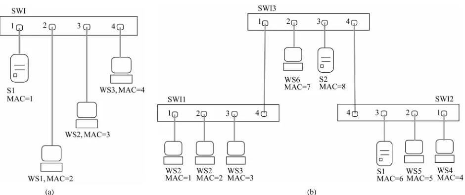
Most widespread topologies of Ethernet are the star shown in Figure 1(a) and the tree shown in Figure 1(b). Star topology is the simplest; it is constituted by single switch (SWI) as well as a stack of switches logically considered as a single switch. To each port of switch only terminal devices are attached. In the tree-like to- pology, there are connections between switches, which are named by uplinks. In such a network the frame passes a few switches on its way to a target device and in the general case each switch has to know all the MAC-ad- dresses of the network. In this study, we do not consider more complex topologies with duplicated paths between devices because these topologies require modeling the spanning tree procedures stipulated by standard IEEE 802.1 D.

To represent realistic traffic we consider an informa- tion system, which uses the network. As a rule, for real- time applications such as technological processes control, there is the primary information system. For instance, Figure 1 represents the networks of railway dispatch centers, supplied with CAM system GID-Ural [8]. On the peculiarities of traffic, we distinguish workstations (WS), which generates requests and servers (S), which executes requests and send responses to workstations. We consider only two-way handshake “request-response” in such an interaction but more complicated protocols may be implemented also.

3. Model of Switched Network

3.1. The Overview of Colored Petri Nets

(a) (b)

Figure 1. Topologies of network. (a) LAN1; (b) LAN2.

Besides CPN Tools colored Petri nets were imple- mented in such well known software as Design/CPN, Helena, Miss-RdP and applied successfully in such areas as networking, protocols’ verification, trains’ traffic con- trol, military operations planning, vehicles control, satel- lite communications and aeronautics.

as natural numbers. For a finite set of numbers a vivid its representation via colors was possible.

CPN Tools [3] uses special kind of colored Petri nets [2] in which tokens are elements of an abstract data type but data types are traditionally named by colors. For de- scription of colors and attributes of places, transitions and arcs CPN ML language is used. The tokens of a place (marking of a place) are represented by multiset; an element belongs to a multiset with a given multiplicity (in a definite number of copies). The multisets are repre- sented by expressions of the following form: k1`e1 ++ k2`e2 ++ …++kl`el, where ki is the multiplicity of ele- ment ei.

3.2. Description of Model

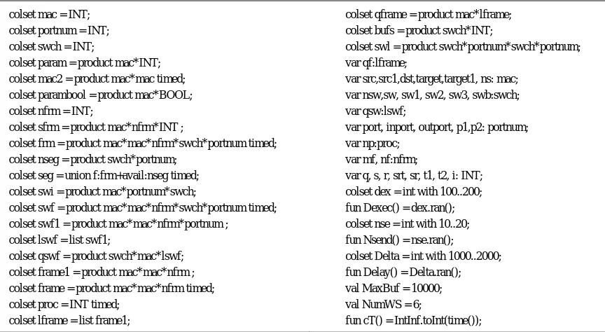
A parametric colored Petri net model of a switched net- work is represented in Figures 2-6. The initial parame-ters correspond to the network structural scheme shown in Figure 1(b). The main page of the model (Figure 2) employs four subpages corresponding to switches SW

(Figure 3), workstations WS (Figure 4), servers S (Fig- ure 5), and measuring fragments MEA (Figure 6); dec- larations are represented in Table 1.

A place possesses a name, color, initial marking and a current marking. A transition possesses a name, guard and time delay. The input arc of a transition has an in- scription defining the pattern for token extraction. The output arc of a transition has an inscription defining the pattern for creation of tokens. The guard constitutes a predicate, which defines the condition for transition’s firing.

In the comparison with the previously presented model [5], the parametric model (Figure 2) is invariant with respect to the networks’ topology. Each page of the model represents all the devices of the same type. For instance, the page SW reflects all the switches of a given network. The solution was obtained on the base of a spe- cial tag, which accomplishes merely each element of the model. The tag uniquely defines the segment of a net- work, which target devices are attached to, with two fields: the number of switch and the number of a switch’s port. The only exception is a segment, which connects a pair of switches. Such a segment has dupli- cated notation with respect to the upper and lower switches, which it is attached to. The following elements of model are labeled with tags: frames, records of switching table and tokens of a segments’ availability. To model times, special timed multisets of the form

e@t are used. It means that token e may be used only after instance t of the model time. In such a notation, @ + d represents the delay with the duration d. Delays may be assigned to transitions as well as to individual tokens.

The dynamics of the net consists in moving the tokens as the result of transitions’ firings. Transition is fireable (permitted) if there are tokens in its input places, which satisfies both the inscriptions of arcs and the guard. At firing, transition extracts tokens from its input places and puts new tokens, constructed according to the rules of output arcs’ inscriptions, into its output places. All the output tokens are delayed with the transition’s firing de- lay.

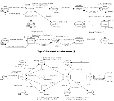
Servers

S Workstations

WS

swithes SW

AttachT 1`(1,1,1)++1`(2,2,1)++1`(3,31`(4,1,2)++1`(5,2,2)++1`(6,3 1`(7,2,3)++1`(8,3,3) swi

inPorts 1`avail(1,1)++1`avail(1,2)++1`avail(1,3)++ 1`avail(1,4)++1`avail(2,1)++1`avail(2,2)++ 1`avail(2,3)++1`avail(2,4)++1`avail(3,1)++ 1`avail(3,2)++1`avail(3,3)++1`avail(3,4)

outPorts 1`avail(1,1)++1`avail(1,2)++1`avail(1,3)++ 1`avail(1,4)++1`avail(2,1)++1`avail(2,2)++

seg

1`avail(2,3)++1`avail(2,4)++1`avail(3,1)++ 1`avail(3,2)++1`avail(3,3)++1`avail(3,4)

swl

WS

1`(1,4,3,1)++1`(3,1,1,4)++ 1`(2,4,3,4)++1`(3,4,2,4)

SwichLink

seg SW

S

Figure 2. The main page of the parametric model. Table. 1. Descriptions of colors, variables and functions.

colset mac = INT; T;

ct mac*INT; ed;

t mac*nfrm*INT ;

ch*portnum timed;

ed;

*portnum timed;

ch*mac*lswf;

ed;

;

colset qframe = product mac*lframe;

*swch*portnum;

target,target1, ns: mac;

outport, p1,p2: portnum;

m;

t1, t2, i: INT;

00..2000;

nt(time()); colset portnum = IN

colset swch = INT; colset param = produ

colset mac2 = product mac*mac tim colset parambool = product mac*BOOL; colset nfrm = INT;

colset sfrm = produc

colset frm = product mac*mac*nfrm*sw colset nseg = product swch*portnum; colset seg = union f:frm+avail:nseg tim colset swi = product mac*portnum*swch; colset swf = product mac*mac*nfrm*swch colset swf1 = product mac*mac*nfrm*portnum ; colset lswf = list swf1;

colset qswf = product sw

colset frame1 = product mac*mac*nfrm ; colset frame = product mac*mac*nfrm tim colset proc = INT timed;

colset lframe = list frame1

colset bufs = product swch*INT; colset swl = product swch*portnum var qf:lframe;

var src,src1,dst,

var nsw,sw, sw1, sw2, sw3, swb:swch; var qsw:lswf;

var port, inport, var np:proc; var mf, nf:nfr var q, s, r, srt, sr,

colset dex = int with 100..200; fun Dexec() = dex.ran(); colset nse = int with 10..20; fun Nsend() = nse.ran(); colset Delta = int with 10 fun Delay() = Delta.ran(); val MaxBuf = 10000; val NumWS = 6; fun cT() = IntInf.toI

ons, represented in Table 1. Media Access Control ad- tween them consists in the option timed.

s introduced. It co

ti

dresses (mac), port numbers (portnum), switch numbers (swch), frames’ sequential numbers (nfrm) are repre- sented with integer type. We abstract from the content of a frame and consider only its header. The frame is repre- sented by color frm, which contains destination and source MAC-addresses, sequential number of request used for the calculation of network response time and the tag with number of switch and number of port. It should be mentioned, that only the destination and source ad- dresses correspond to the real fields of an Ethernet frame’s header, remaining variables are artificially added for the purposes of parametric model’s construction and measurement. Auxiliary types frame, frame1 are used inside submodel of server (S); they do not contain the tag with switch and port number. The only difference be-

For the adequate modeling of frames’ transmission through Ethernet segments, color seg i

(nsw,ns,(src,dst,nf,port)::qsw)

avail(sw,inport)

(sw1,p1,sw2,p2) f(src,dst,nf,sw1,outport)

f(src,dst,nf,sw2,p2)

avail(sw3,outport)

swf

bufs swl

seg

seg qbuffer

buffer

(target,port,sw1)

avail(sw,p1) f(src,dst,nf,sw,inport)

@+12 avail(sw1,outport)

f(src,dst,nf,sw,inport) (swb,i)

1`(1,0)++1`(2,0)++1`(3,0)

[dst=target,sw1=sw, swb=sw,i<MaxBuf] (src,dst,nf,sw,port)

(nsw,ns,qsw)

[o ns 1`(1,1,[])++1`(1,2,[])++1`(1,3,[])++1`(1,4,[])++

1`(2,1,[])++1`(2,2,[])++1`(2,3,[])++1`(2,4,[])++

1`(3,1,[])++1`(3,2,[])++1`(3,3,[])++1`(3,4,[]) utport=port,swb=sw1,_w=sw1]

(src,dst,nf,sw,port)

swtab @+5

swi

1`(1,1,1)++1`(2,2,1)++1`(3,3,1)++ 1`(4,4,1)++1`(5,4,1)++1`(6,4,1)++ 1`(7,4,1)++1`(8,4,1)++1`(1,4,2)++ 1`(2,4,2)++1`(3,4,2)++1`(4,1,2)++ 1`(5,2,2)++1`(6,3,2)++1`(7,4,2)++ 1`(8,4,2)++1`(1,1,3)++1`(2,1,3)++ 1`(3,1,3)++1`(4,4,3)++1`(5,4,3)++ 1`(6,4,3)++1`(7,2,3)++1`(8,3,3) (nsw,ns,qsw)

SwichLinkI/OI/O [nsw=sw,ns=port ]

(swb,i) buffersize

put outPorts I/OI/O

@+5

(swb,i-1)

(swb,i+1)

get

uplink

[sw1=sw,p1=inport, sw2=sw3,p2=outport] addbuf

inPorts I/O I/O (nsw,ns,qsw^^[(src,dst,nf,port)])

qswf

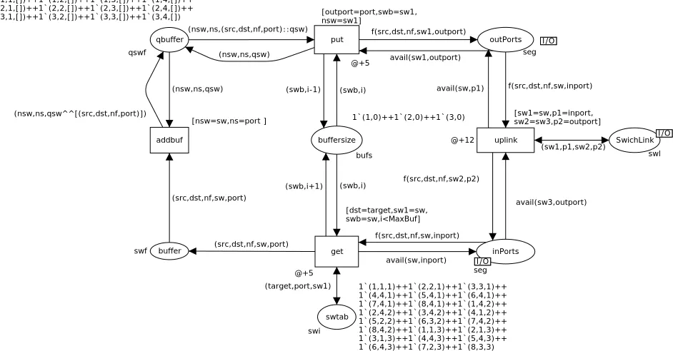
Figure. 3. Parametric model of switches (SW).

and number of port. In the initial m

parate label for each segment of network. Before

egments, which connect switches, have a pair of

. It co

ith place qbuffer. Each token in this place models the queue to a given port of a given switch.

ent, w

requests are repre- se

arking we have a switch represented w se

transmission of a frame into the segment, each device is waiting for the corresponding avail label and removes this label replacing it by frame. At the acceptance of the frame by device, it is replaced by the corresponding avail

label. The described procedure guarantees that not more than one frame is being transmitted in each segment at the same time.

The page SW (Figure 3) represents all the switches. Note that, s

labels avail with the respect to each switch. To proc- ess this special case the transition uplink is introduced. It provides the transformation of the segment’s number and moves the frame from the place outPorts for source switch to the place inPorts for destination switch. Place

SwitchLink contains the information about the connec- tions among switches represented with color swl. This color includes definitions for the both ends of connection: the number of the switch and the number of the port.

The color swi is used for the description of static switching tables for all the switches of the network

nsists of usual fields of switching table such as MAC-address and port’s number accomplished with the tag containing the number of switch. All the switching tables are represented with the marking of a single place

swtab. Using records from this place switch assigns the output port’s number for arrived frame via the transition

get. Then frame is allocated in the internal buffer of

The record of the queue is described with color swf1 (swf), whereas the queue is represented with the color qswf. The frame is moved to the output segment of switch via tran- sition put. Place buffersize counts the number of occupied slots of frames’ buffer for each switch. The limits of buffer sizes are checked in the guard of transition get.

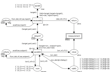
The page WS (Figure 4) represents all the workstations, whereas the page S (Figure 5) represents all the servers. It’s implemented in such a way that each host listens for the frame with its destination address only in the segm

hich it is attached to. A simple description of network’s topology is situated in the place AttachT. Color swi is used for assignment of Ehternet segment for each MAC-address; segment is given by the pair: number of switch and number of port. It should be noted that, to- gether with the marking of the place SwitchLink place

AttachT gives the complete information about network’s topology. Place AttachT is used either at listening a seg- ment for receiving a frame via transitions receive* (re- ceiveWS, receiveS) or at uttering a frame into segment via transitions send* (sendWS, sendS).

We consider a simple two-way handshake as the pro- tocol of client-server interaction. The workstation sends a request; the server executes the request and sends an answer. Delays between the client’s

sendWS

[target=src, outport=port, src1=src,sw1=sw]

sfrm

sfrm

param mac2

mac 1`1++1`2++1`3++

1`4++1`5++1`7 ownWS

swi

seg seg

(src,dst) inPorts

I/O I/O

num outPorts

I/O I/O

rqWS return

nSnd measurement MEA

MEA

avail(sw,outport)

f(src,dst,nf,sw,outport) avail(sw,inport)

target1 _{[dst=target,target=target1,} sw1=sw, inport=port]

(target,port,sw1)

@+14

@+14 receiveWS f(src,dst,mf,sw,inport)

(src1,nf+1) (src1,nf)

1`(1,1)++1`(2,1)++ 1`(3,1)++1`(4,1)++ 1`(5,1)++1`(7,1)

(target,port,sw1)

AttachT I/O I/O

(src,dst)@+Delay() 1`(1,6)@+Delay()++1`(1,8)@+De_{1`(2,6)@+Delay()++1`(2,8)@+De} 1`(3,6)@+Delay()++1`(3,8)@+De 1`(4,6)@+Delay()++1`(4,8)@+De 1`(5,6)@+Delay()++1`(5,8)@+De 1`(7,6)@+Delay()++1`(7,8)@+De (src,nf,cT())

(dst,mf,cT())

Figure 4. Parametric model of workstations (WS).

with function Dexec(). We consider a request consisting of a single frame and the response

om number of frames represented with function Nsend().

ing the servers, which they re

queues represented with place qreply. Each token in place he output queue of a given server. Then frames are transmitted into segment, which the

r and workstation, we enumerate the requests vi

consisting of a ran- qreply corresponds to t d

Moreover, we suppose that each server has a few proc- essors defined by the marking of place processor. This place contains the number of processors for a given MAC-addresses of servers.

Let us consider the trace of client-server interaction to study the model more thoroughly. Place rqWS defines the activity of workstations point

quire. Color mac2 is used to define the pairs: MAC- address of workstation, MAC-address of server. After uttering the frame of request into the segment via transi- tion sendWS the pair is frozen on the duration given with function Delay(). Through switches the frame arrives into segment, which the target server is attached to. The server reads the frame via the transition receiveS and puts it into the input queue of the server via transition addqreq. Each token of the place qrequest represents a queue to the cor- responding server. After the execution of the request via transition exec, obtained reply consisting of Nsend() frames is situated into place reply. Note that, at construc- tion the frames of reply, we change the positions of the source and destination addresses in the frame’s header to provide the backward transmission from server to re- quired workstation. All the replies are moved into output

server is attached to, via transition sendS. Segment is de- termined on the base of information about network’s to- pology situated in place AttachT. Through switches the frame arrives into a segment, which the required work- station is attached to, and is accepted via transition re- ceiveWS.

For the calculation of Network Response Time (NRT) we use the special measuring fragment of colored Petri net

MEA (Figure 6). Elements of this fragment do not model any real software of hardware; they are used for the pur- poses of measurement only. For each pair of communi- cating serve

(src,dst,nf) target1 sendS [ns=src] @+Dexec() frame 1`6++1`8 proc fr seg ame 1`6++1`8 mac seg inPorts I/O I/O outPorts I/O I/O receiveS AttachT I/O I/O qreply qrequest exec f(src,dst,nf,sw1,inport) avail(sw1,port) [dst=target, target=target1, sw1=sw,inport=port] (src,dst,nf) avail(sw,outport) f(src,dst,nf,sw,outport) swi (target,port,sw1) (target,port,sw1) @+14 [target=src, outport=port, sw1=sw] (ns,(src,dst,nf)::qf) (ns,qf)

request src,dst,nf)

1`(6,[])++1`(8,[]) ( [ns=dst] qframe (ns,qf^^[(src,dst,nf)]) (ns, qf) (ns,qf) [dst=np] np reply addqrep (ns,qf^^[(src,dst,nf)]) @+14 1`(6,[])++1`(8,[]) addqreq processor qframe ownS Nsend()`(dst,src,nf) (ns,(src,dst,nf)::qf) (ns,qf)

Figure 5. Parametric model of servers (S).

sr

srt div NumWS

true true

srt-r+(s div q) srt

(src1,s div q) (src1,r) (src1,true) (src1,s) (src1,q) (src1,q+1) (src1,q) (src1,s+(t2-t1)) (src1,s) (src1,true) (src,nf,t2-t1) (src,nf,t1) (dst,mf,t2) Culc1 Culc IsFirst [dst=src,nf=mf, src=src1] AvrNRT 0 INT new1 BOOL sumall 0 INT NRTime 1`(1,0)++1`(2,0)++1`(3,0)++ 1`(4,0)++1`(5,0)++1`(7,0) param quan 1`(1,0)++1`(2,0)++1`(3,0)++ 1`(4,0)++1`(5,0)++1`(7,0) param 1`(1,0)++1`(2,0)++1`(3,0)++ 1`(4,0)++1`(5,0)++1`(7,0) param nSnd sum In _sfrm NRTs sfrm new parambool return In _sfrm In In srt

Figure 6. Measuring fragment for the network response time evaluation (MEA).

For debugging purposes response times for all the re- quests are stored in place NRTs. But we are interested

ave

art of the measuring fragment calculates the average

e topology of networks

AttachT and

swi enumerates MAC-

addresses of terminal devices attached to each port o each switch. Note that, the hubs usage may be repre ttached to the same port. Links between switches (uplinks) are represented y the marking of place SwitchLink with color swl. Color especially in the

p

rage response times. The residuary sented by a few MAC-addresses a

response times for each workstation (place NRtime) via transition Culc and the total average response time for the entire network (place AvrNRT) via transition Culc1.

4. Parameters of Model

.1. Topological Parameters 4

he primary information about th T

is represented as the marking of places

SwitchLink. Place AttachT of color

f -

b

swl describes both ends of link as a pair: the number of switch and the number of port. For modeling conven- ience each link is described twice for each of the two possible directions of the frames’ transmission. For in- stance, for the network drawn in Figure 1(a) the marking of place SwitchLink would be empty and marking of place AttachT would be equal to: 1`(1,1,1) ++ 1`(2,2,1) ++ 1`(3,3,1) ++ 1`(4,4,1).

wn in Figure 1(a) the m

er both the network hardware such as switches an

th respect this size of frame. In the data sheets of switches either r in gigabits per sec- nd is written. For instance, switch Intel SS101TX4EU

. The performance of

e 2, MTU is equal to 10 ms.

affic control. weakly on the per-

directly in timed tervals as uniformly distributed random value given by

token with the ad

cur- . The next moment of model time is

g to the list of future events. place swtab with color swi. Since each switch contains

information about each known terminal device, there are a few records for a chosen MAC-address; the number of these records corresponds to the number of switches. For instance, for the network dra

arking of place swtab would be the same as the mark- ing of place AttachT. Note that, for an arbitrary network with the star topology, the markings of places AttachT

and swtab coincide and marking of place SwitchLink is empty.

Thus, places AttachT and SwitchLink contain the en- coding of the network tree: leaves of the tree are men- tioned in place AttachT while internal nodes (including the root) are mentioned in place SwitchLink.

4.2. Parameters of Hardware

We consid

d network adapters, and the terminal hardware such as workstations and servers. For convenience we consider frames of maximal length with useful capacity of 1500 Kbytes and express parameters of the model wi

to

performance in frames per second o o

possesses the performance of about 10000 packets per second [10]. From this value we calculate the average time of one frame processing as 100 ms, which corre- sponds to the total delay of transitions get and put. An ideal performance of the network is defined by its stan- dard, for instance the minimal time of 1500 byte frame transmission accounting for an additional size of header, preamble and standard delay between frames is equal to 123 ms for 100 Mbps Ethernet. Furthermore in calculations we use the total length of a frame equaling to 12304 bits. Real Ethernet adapters provide a lesser performance; an evaluation is presented in [10]. For instance, the card Intel Ether Express PRO/100+ provide actual perform- ance in one direction about 92,1 Mbps; this corresponds to the delay about 140 ms. This value represents the de- lays of transitions send*, receive*.

Performances of workstations and servers have dif- ferent influences on the parameters of the model. The performance of a workstation is not essential for the pe- riod of requests, which is determined mainly by the characteristics of information system and relays on slow by thousands times man-machine interaction. Therefore we consider the period of requests completely defined by parameters of an information system

a server has a direct influence on the time of a re- quest’s execution. The average time of request execution (transition exec) may be either measured for each type of hardware on the test sequences of requests or calculated

on the information about the number of abstract opera- tions and performance. In both mentioned cases it relays on parameters of software and will be discussed in the next section.

Note that, the modeling system maintains time in its internal units MTU (Model Time Unit). Before modeling we have to express all the timed values in MTU using the scaling of times. As 1 MTU we may choose the smallest time value among all the parameters but for the purposes of future representation of faster devices it is appreciated to choose more little value. For instance, in the model shown in Figur

4.3. Parameters of Software

We consider as the primary such parameters of software as: the period of workstations’ requests, the average length of request, the average hardness of request’s exe- cution, the average length of response. We study the CAM software GID-Ural [8] of trains’ tr

Since the period of requests depends formance of hardware, we measure it in

function Delay() of range 20-40 s or 2000-4000 MTU. The lengths of requests and responses primarily given with the number of bytes we measure in number of frames with maximal length; they are also represented as uniformly distributed random values. For instance, re- quest length 1-1,5 Kb is represented with one frame, re- sponse length 15-30 Kb is represented with a random function Nsend() of range 10-20 frames.

We estimated the average time of request execution on test sequences of requests for the HP Brio server; it equals to 1-2 s and it is represented in the model with the uni- formly distributed random function Dexec() of the range 100-200 MTU. Moreover, the model reflects the informa- tion links between the workstation and the servers given by the table of workstations’ activity represented with the marking of place rqWS, which contain a

dress of the workstation and the address of the server for each the interacting pair of terminal devices. In our example each workstation interacts with each server.

5. Simulation

For the debugging of models CPN Tools provides the step-by-step mode of simulation with visual displaying of all the events at the current moment of model time. Either one step or a given number of steps may be exe-

uted. It is assumed, that a step corresponds to an oc c

Let us consider the process of a request’s frame trans-

okens is w

h st

S ac- co

f mo

mission from one of workstations to server and re- sponse's frames backwards from server to requested workstation. This delivery loop is the base one for the client-server systems. The initial state of the model is given by Figures 2-6. The current marking of places cre- ated on initial marking is shown inside green rectangles beside corresponding place; the number of t

ritten inside small circles. Clicking on these circles user can show or hide place’s marking. Note that according to the marking of place rqWS generated by random function

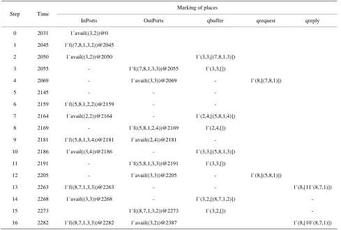
Delay() initial moment of model time is equal to 2031. For compact representation of the simulation process, we use the trace table (Table 2). This table describes states of model at each step. Note that the table contains only base elements of the model, which participate in the frames’ transmitting.

Frame (7,8,1) with request 1 of workstation WS6(mac = 7) sent to server S2 (mac = 8) at step 1, has been deliv- ered to server at 4th step and executed by server at 13t

ep; as the result 12 frames of reply have been generated. Beginning at 13th step the delivery of frames in the op- posite direction is executed. At step 16 the first frame of the reply has been delivered to workstation WS6 and ab-

sorbed by transition receiveWS. It should be noticed, that Table 2 displays also others events taking place in the model. For instance, execution of the request of work- station WS5 (mac = 5) sent to server S2at step 6.

Let us consider in detail the process of frames’ tags modification, since it is the base for the parametric model behavior comprehension. At step 1, tag of re- quest’s frame (3,2) is created by transition sendW

Table 2. Trace o

rding to network’s topology given by place AttachT: MAC address 7 is attached to port 2 of switch 3. After switching at step 3, tag (3,3) is assigned by transition put

because target device with MAC address 8 is attached to port 3 of the same switch 3. Analogous assignment of tags is executed for reply’s frames at steps 13, 15 by transitions sendS, put. More complicated case constitutes the request of WS5 to server S2 because client and server are attached to different switches. Initial tag (2,2) is re- placed by tag (2,4) at step 8 and then at step 9 is over- written with tag (3,4) by transition uplink representing the transmission between switches 2 and 3; the frame is redirected from port 4 output channel of switch 2 to port 4 input channel of switch 3. The assignment of tag (3,3) at step 11 finishes the delivery of request to target device attached to port 3 of switch 3.

del’s behavior.

Marking of places Step Time

InPorts OutPorts qbuffer qrequest qreply

0 2031 1`avail((3,2))@0

1 2045 1`f((7,8,1,3,2))@2045

2 2050 1`avai 2050 1`(3, 3)])

1`f((7,8,1, ))@2055 1`(3 ,[])

1`avail((3,3))@2069 - 1`(8,[(7,8,1)])

1`f((5,8,1, ))@2159

1`avail((2 )@2164 1`(2,4,[ ,1,4)])

1`f((5,8,1, ))@2169 1`(2 [])

1`avail((2 )@2181

1`(8,[(5,8,1)])

1`(8,[11` ,7,1)])

1`avail((3 )@2268 1`(3 )])

1`(3 [])

1`avail((3 )@2387

l((3,2))@ 3,[(7,8,1,

3 2055 - 3,3 ,3

4 2069 -

5 2145 - - -

6 2159 2,2 - -

7 2164 ,2) - (5,8

8 2169 - 2,4 ,4,

9 2181 1`f((5,8,1,3,4))@2181 ,4) -

10 2186 1`avail((3,4))@2186 - 1`(3,3,[(5,8,1,3)])

11 2191 - 1`f((5,8,1,3,3))@2191 1`(3,3,[])

12 2205 - 1`avail((3,3))@2205 -

13 2263 1`f((8,7,1,3,3))@2263 - - (8

14 2268 ,3) - ,2,[(8,7,1,2 -

15 2273 1`f((8,7,1,3,2))@2273 ,2, -

A e tra T omplete loop f

clien er for th air of MAC

(7,8 et us c der the netw rk response t

alc tion. The time as s

l

ep- y-step simulation as well as automatic slow simulation ynamics for a speci- ed number of steps. For the accumulation of statistical

d in is the existence f the steady-state mode. For the parameters of the

teady-state ode, which may be observed for instance using Table 3.

ow of the table, this is concerned with the

avior of the etwork in the steady-state mode. We are interested in he variations of NRT with respect to different network

T tate mode twork behavior.

STE 1 000 10 000 100 000 00 000 s th ce table ( able 2) contains c o

t-serv ), l

interaction onsi

e p o

addresses ime (NRT) c

p

ula of request (2031) w aved in the ace nSnd and the time of reply’s arrival (2273) is saved in place return; the sequential number of request is indi- cated by field nf of frame. After reply’s arrival, transition

IsFirst recognizes the first frame of reply and starts the process of response time’s recalculation. Place Sum con- tains (7,242), that means: the sum of response times for workstation with MAC address 7 is equal to 242 (2273- 2031). Place quan contains (7,1): number of responded requests for workstation with MAC address 7 is equal to 1. Place new runs the recalculating of average NRT for each workstation by transition Calc, which are stored in place NRTime: (7,242). Note that, place AvrNRT contains inconsistent values only at startup interval of time be- fore the arrival of responses for each workstation.

6. Performance Evaluation

For the debugging of models, CPN Tools proposes st b

with the visualization of Petri net d fi

information, a special mode of fast simulation without visualization is used. It provides the consideration of huge enough intervals of real time.

6.1. Conditions for Steady-State Mode

The major question we are intereste o

model shown in Figure 2-6 we obtain the s m

After model time instance 100000 the value of NRT is stabilized and does not change any more. This interval corresponds to one and a half second of real time. Ob- tained network response time equaling to 392 MTU or about 4 s satisfies the requirements of train traffic con- trol [8].

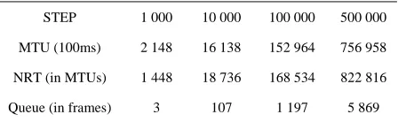
Table 4 illustrates the absence of the steady-state mode for the 10 Mbps network. The value of NRT is growing in time. As we may easily conclude from the bottom r

growth of frames’ output queues in servers.

6.2. Evaluation of Characteristics

Furthermore we are investigating the beh n

t

able 3. Steady-s of ne

P 1 0

MTU (10ms 2 162 16 215 152

92 392

) 880 1 512 989

NRT (in MTUs) 689 456 3

Table 4. Absence of steady-state mode for 10 Mbps net- work.

00 STEP 1 000 10 000 100 000 500 0

MT ms) 8

) 8

) 7

U (100 2 14 16 138 152 964 756 958

NRT (in MTUs 1 44 18 736 168 534 822 816

Queue (in frames 3 107 1 19 5 869

and computer hardware (Figure 7). In this study, we try four 100 Mbps network adapters Intel Express PRO/100+, Allied Telesyn AT2500, Butterfly, Cnet CNPro 200 with

charac s given 0] l e P

Bri c, S rig n i e

estim p ters erfo es

pe ze fer T m

gr 7(a) rrespo to In 101 U

nd 3Com Switch 4005, intermediate points represent

k.

Et

teristic in [1 as wel as four s rvers H o, Power Ma

ated with two GI O arame

in, Su : the p

Fire. Sw rmance in

tches ar fram r second and si of buf in Kb. he extre e ends of aphs in Figure co nds tel SS TX4E a

switches of Cisco Catalist series.

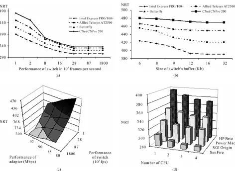
Figure 7(a) shows that switches choice with perform- ance greater than 28104 frames per second, which cor- responds to switch Catalist 2900XL, does not lead to a decrease of NRT. Figure 7(b) shows that only switches’ buffers lesser than 16Kb have influence on NRT. In Fig- ure 7(c) the total influence of network hardware such as switches and network adapters on NRT is illustrated; the surface has the form of an inclined strip. Figure 7(d) contains the diagram, which illustrates the variation of NRT on servers’ hardware and number of processors. There is no merely difference between NRT for servers with more than two processors.

Constructed graphs may be applied for solving the task of the optimal network’s hardware choice. Two ba- sic characteristics, such as NRT and the cost of hardware, may be considered either as the criteria or as the bound.

Note that, the results obtained with the parametric and nonparametric [5] models coincide but the parametric model does not require the editing of model structure for each given network: only the encoded network tree is put into places AttachT and SwitchLin

7. Conclusions

(a) (b)

(c) (d)

Figure 7. Variation of the network response time (NRT). (a) On performance of switches; (b) On size of buffer; (c) On net-work’s hardware; (d) On server’s hardware.

servers and switches. The model has a fixed number of nodes for an arbitrary given

As the structure of a given network is a parameter

8.

ensor Networks Using GTNetS,” Proceedings of 12th Annual Meeting of the IEEE/ACM International Modeling, Analysis, and Simulation o Telecommunication Systems, Volendam, 5-7 October 2004, pp. 375-382.

sis Methods and Practical Use,” Springer-Verlag, Berlin,

Petri Nets,” LNCS 2031: Tools and Algorithms for the

n of 12th Annual

Meet-2003.12.004 network and, moreover, it Vol. 1-3, 1997. implements the evaluation of network response time as

the major parameter of network’s performance.

[3] M. Beaudouin-Lafon, W. E. Mackay, M. Jensen, et al., “CPN Tools: A Tool for Editing and Simulating Coloured

represented by the marking of dedicated places, it pro- vides an easy reuse of the model which could be embed- ded into networks’ CAD systems.

The performance evaluation for the network of the railway dispatcher center was implemented. The ob- tained results may be used at the development of real- time systems.

References

[1] X. Zhang and G. F. Riley, “Bluetooth Simulations for Wireless S

pp.

f

Oc

Symposium on Computer and

[2] K. Jensen, “Colored Petri Nets—Basic Concepts,

Analy-Construction and Analysis of Systems, 2001, pp. 574-580. http://www.daimi.au.dk/CPNTools

[4] D. A. Zaitsev, “Verification of Protocol TCP via Decom- position of Petri Net Model into Functional Subnets,”

Proceedings of the Poster Sessio

ing of the IEEE/ACM International Symposium on Mod-eling, Analysis, and Simulation of Computer and Tele-communication Systems, Volendam, 5-7 October 2004,

73-75.

[5] D. A. Zaitsev, “An Evaluation of Network Response Time Using a Coloured Petri Net Model of Switched LAN,” 5th Workshop and Tutorial on Practical Use of Coloured Petri Nets and the CPN Tools, Aarhus, 8-11

tober 2004, pp. 157-167.

ations), Vol. 46, No. 2, 2004, pp. 56-60. apo-[7] D. A. Zaitsev and T. R. Shmeleva, “Modeling of Switched

Local Area Networks by Colored Petri Nets,” Zviazok

(Communic

[8] H. S. Zyabirov, G. A. Kuznetsov, F. A. Shevelev, et al., “Automated System for Operative Control of Exploita-tion Work GID Ural-VNIIZT,” Railway Transport, No. 2,

2003, pp. 36-45.

[9] R. Breyer and S. Riley, “Switched, Fast, and Gigabit Ethernet,” MacMillan Technical Publications, Indian lis, 1999, pp. 1-618.