Valid confidence intervals for post model selection predictors

Munich Personal RePEc Archive

Valid confidence intervals for

post-model-selection predictors

Bachoc, Francois and Leeb, Hannes and Pötscher, Benedikt

M.

Department of Mathematics, University Paul Sabatier, Department

of Statistics, University of Vienna, Department of Statistics,

University of Vienna

December 2014

Online at

https://mpra.ub.uni-muenchen.de/76453/

Valid con…dence intervals for post-model-selection predictors

François Bachoc*, Hannes Leeb**, and Benedikt M. Pötscher** *Department of Mathematics, University Paul Sabatier

**Department of Statistics, University of Vienna

First version: December 2014 This version: December 2016

Abstract

We consider inference post-model-selection in linear regression. In this setting, Berk et al. (2013a) recently introduced a class of con…dence sets, the so-called PoSI intervals, that cover a certain non-standard quantity of interest with a user-speci…ed minimal cov-erage probability, irrespective of the model selection procedure that is being used. In this paper, we generalize the PoSI intervals to con…dence intervals for post-model-selection predictors.

AMS Mathematics Subject Classification 2010: 62F25, 62J05.

Keywords: Inference post-model-selection, con…dence intervals, optimal post-model-selection predictors, non-standard targets, linear regression.

1

Introduction and overview

Prediction following model selection is obviously also of great importance. In the case where the selected model is misspeci…ed, parameter estimates are typically biased or at least di¢cult to interpret; cf. Remark 2.7. But even a misspeci…ed model may perform well for prediction. In particular, Greenshtein and Ritov (2004) derive, under appropriate sparsity assumptions, feasible predictors that asymptotically perform as well as the (infeasible) best candidate predictor even if the available number of explanatory variables by far exceeds the sample size. These feasible predictors are also covered by the results in the present paper, among others. Like Greenshtein and Ritov (2004), our analysis does not rely on the assump-tion that the true data generating model is among the candidates for model selecassump-tion. We develop con…dence intervals for such predictors, that are easy to interpret and that are op-timal in an appropriate sense; cf. Remarks 2.7(ii), 2.8, and 3.2, as well as Greenshtein and Ritov (2004). A further rationale for extending the PoSI-approach of Berk et al. (2013a) to problems related to prediction is that this framework seems to provide a more natural habitat for considering non-standard targets; see the discussion in Remark 2.1 of Leeb et al. (2015) as well as in Remarks 2.7 and 3.1 given further below.

The crucial feature of the approach of Berk et al. (2013a) is that the coverage target, i.e., the quantity for which a con…dence set is desired, isnot the standard target, i.e., the parameter in an overall model (or components thereof), but a non-standard quantity of interest that depends on the selected model and thus on the data. This non-standard quantity of interest is denoted by (n_^)

M throughout the paper (cf. Section 2 for details). Here M^ stands for the (data-dependent) model chosen by the model selector andnstands for sample size. The non-standard target (n_^)

M provides a certain vector of regression coe¢cients for those explanatory variables that are ‘active’ in the model M^ (more precisely, (n_^)

M represents the coe¢cients of the projection of the expected value vector of the dependent variable on the space spanned by the regressors included inM^); for a precise de…nition see eqs. (3) and (4) in Section 2.

For a new set of explanatory variables x0, we …rst extend the PoSI-approach to obtain

con…dence intervals for the predictor x0₀[ ^M] (n_^)

M . Here, x0[ ^M]denotes the set of explanatory variables fromx0that correspond to the ‘active’ regressors in the modelM^. We callx00[ ^M]

(n) ^

M the design-dependent (non-standard) coverage target, because di¤erent design matrices in the training data typically result in di¤erent values of x0₀[ ^M] (n_^)

M even if both training data sets lead to selection of the same model M^. We construct PoSI con…dence intervals for

x0

0[ ^M] (n)

^

M that guarantee a user-speci…ed minimal coverage probability, irrespective of the model selector that is being used. The design-dependent coverage target minimizes a certain ‘in-sample’ prediction error; cf. Remark 2.8. However, when the goal is to predict a new response corresponding to a new vectorx0 of explanatory variables, this ‘in-sample’ optimality

property may have little relevance and thus the focus on covering the design-dependent target

x0₀[ ^M] (_^n)

M may be debatable.

In view of this, we next consider an alternative coverage target that depends on the selected model but not on the training data otherwise, and that we denote by x0

0[ ^M] (?)

^

M. We call

x0₀[ ^M] (_^?)

prediction error, over all (infeasible) predictors of a future response y0 that are of the form

x0

0[ ^M] ( ^M), when x0 and the row-vectors of X are sampled from the same distribution; cf.

Remark 3.2. In particular, this target does not su¤er from the issues that plague the design-dependent coverage target, as discussed at the end of the preceding paragraph. Certain optimality properties of a feasible counterpart of x0

0[ ^M] (?)

^

M are derived in Greenshtein and Ritov (2004), for a particular model selectorM^ and under appropriate sparsity assumptions; a target closely related tox0₀[ ^M] (?_^)

M is also studied in Leeb (2009). For a large class of model selectors, we show that the PoSI con…dence intervals constructed earlier also cover the design-independent coverage target with minimal coverage probability not below the user-speci…ed nominal level asymptotically. In that sense, the PoSI con…dence intervals are approximately valid for the targetx0₀[ ^M] (?_^)

M, irrespective of the model selectorM^ in that class. In simulations we …nd that our asymptotic result is representative of the …nite-sample situation even for moderate sample sizes.

When extending the PoSI-approach to con…dence intervals for both the design-dependent and the design-independent coverage target, i.e., for both x0

0[ ^M] (n)

^

M and x

0

0[ ^M] (?)

^

M, we …nd that the resulting intervals necessarily depend not only onx0[ ^M]but also on those components

ofx0 that are ‘in-active’ in the modelM^. This may appear surprising at …rst sight but turns

out to be inherent to the PoSI-approach (because of the need to take the maximum over all modelsM in (10)). In any case, this is problematic in situations when, after having selected a given model, only the ‘active’ components of x0 are observed, e.g., in situations where

observations are costly and model selection is carried out also with the goal of reducing cost by not having to observe irrelevant components of x0. To resolve this, we also develop PoSI

con…dence intervals that depend on the ‘active’ variables x0[ ^M] only. These intervals are

obtained by maximizing over all inactive variables and are hence larger than the intervals for the case where x0 is known entirely. In simulations, we …nd that the excess width of these

intervals is moderate. We also provide analytic results regarding the excess width of these intervals in an asymptotic setting where the number of regressors goes to in…nity, see Section 2.4.

Inference post-model-selection is currently a very active area of research and we can only give a selection of work relevant for, or related to, this paper. Contemporary analyses of con…dence sets for (components of) the true parameter of the underlying model include An-drews and Guggenberger (2009), Kabaila and Leeb (2006), Leeb and Pötscher (2005), Pötscher (2009), Pötscher and Schneider (2010), and Schneider (2016). These references also point to numerous earlier results. Also, the work of Lockhart et al. (2014), Wasserman and Roeder (2009), and Wasserman (2014) should be mentioned here. For the LASSO, in particular, a de-sparsifying method has recently been developed by Belloni et al. (2011, 2014), van de Geer et al. (2014), and Zhang and Zhang (2014). Another strand of literature that, like the PoSI approach, also focuses on (n_^)

M as the quantity of interest, is developed in Fithian et al. (2015), Lee et al. (2016), Lee and Taylor (2014), Tian and Taylor (2015), Tibshirani et al. (2015), and Tibshirani et al. (2016): In these papers, con…dence sets for (_^n)

intervals obtained in these papers are speci…c to the model selection procedure used (the LASSO, in particular, being considered in these references) and generally rely on certain geo-metric properties of the speci…c model selection procedure under consideration. In simulation experiments, we compare the con…dence intervals proposed in these references with the inter-vals developed here and observe some interesting phenomena, see Section 4.3. As prompted by a referee, we point out here that in the presence of a large number of regressors PoSI intervals (including intervals considered in the present paper) typically are computationally more burdensome than the con…dence intervals proposed in Lee et al. (2016) for the LASSO with a …xed value for the tuning parameter; see, however, also the discussion towards the end of Section 4.3.

The rest of the paper is organized as follows. In Section 2, we introduce the models, the model-selection procedures, the design-dependent target, and the PoSI con…dence intervals for both the case where all explanatory variables inx0 are observed and the case where only the

components ofx0 corresponding to the ‘active’ explanatory variables are available; moreover,

we analyze properties of these intervals in an asymptotic framework where the model dimen-sion increases; cf. Section 2.4. In Section 3, we present the design-independent target and show that the PoSI con…dence intervals introduced earlier also cover the design-independent target, with minimal coverage probability not below the nominal one asymptotically when sample size increases. The results of a numerical study are reported in Section 4. Conclusions are drawn in Section 5. Appendix A contains some comments on the assumptions made on the errors variance. The proofs of the results in Sections 2 and 3 are given in Appendices B and C. Appendix D contains some comments on and extensions of the results in Section 3. In Appendix E we describe algorithms for computing the PoSI con…dence intervals, that are comparable with those proposed by Berk et al. (2013a) in terms of computational complexity. Finally, Appendix F contains details concerning the numerical calculations used for the results in Section 4.

2

Con…dence intervals for the design-dependent non-standard

target

2.1 The framework

Consider the model

Y = +U (1)

where ₂Rn _{is unknown and U follows an N 0;} 2_I

We consider …tting (potentially misspeci…ed) linear models with design matrices that are obtained by deleting columns fromX. Such a model will be represented by M, a subset of

f1; :::; p_g, where the elements of M index the columns of X that are retained. We use the following notation: ForM _f1; :::; p_g, we writeMc for the complement ofM in_f1; :::; p_g. It proves useful to allowM to be the empty set. We write_jM_j for the cardinality ofM. With

m=_jM_j, let us write M =_fj1; :::; jmgin casem 1. ForM 6=?and for anl pmatrixT,

l 1, letT[M]be the matrix of dimensionl mobtained fromT by retaining only the columns ofT with indices j₂M and deleting all others; ifM =?we setT[M] = 0₂Rl_{. In abuse of} notation we shall, for ap 1 vectorv, writev[M]for(v0[M])0, i.e., v[M] = (vj1; :::; vjm)

0 _for

m 1andv[M] = 0₂Rin caseM =?. For a given model M, we denote the corresponding least squares estimator by ^_M, i.e.,

^

M = X[M]0X[M]

1

X[M]0Y; (2)

where the inverse is to be interpreted as the Moore-Penrose inverse in case X[M] does not have full column rank. For any given modelM the corresponding least squares estimator ^_M is obviously an unbiased estimator of

(n)

M = X[M]

0_X[M] 1

X[M]0 : (3)

Note that ^_M as well as (_Mn) reduce to0 in case M =?.

As in Berk et al. (2013a) we further assume that, as an estimator for 2, we have available an (observable) random variable ^2 that is independent of PXY and that is distributed as

2_{=rtimes a chi-square distributed random variable with r degrees of freedom (1 r <1),}

withPX denoting orthogonal projection on the column space ofX. This assumption is always satis…ed in the important special case where one assumes thatd < n and ₂span(X) hold, upon choosing for^2 the standard residual variance estimator obtained from regressingY on

Xand upon settingr =n d. However, otherwise it is not an innocuous assumption at all and this is further discussed in Appendix A. Observe that our assumption allows for estimators ^2 that not only depend onY andX, but possibly also on other observable random variables (e.g., additional data). The joint distribution ofY and ^2 depends on and as well as on sample sizenand will be denoted by Pn; ; (see also Appendix D.4).

satisfying our assumptions is the collection of all full-rank submodels of _f1; :::; p_g (enlarged by the empty model) provided that no column of X is zero; of course, there are many other examples, see, e.g., the list in Section 4.5 of Berk et al. (2013a).

A model selection procedure M^ is now a (measurable) rule that associates with every (X; Y;^2) a (possibly empty) model M^(X; Y;^2) _{2 M}. In the following we shall, in abuse of notation, often write M^ for M^(X; Y;^2). Allowing explicitly dependence of M^ on ^2 is only relevant in case ^2 depends on extraneous data beyond (X; Y) and the model selection procedure actually makes use of ^2. [We note here that in principle we could have allowed

^

M to depend on further extraneous data, in which casePn; ; would have to be rede…ned as the joint distribution ofY, ^2, and this further extraneous data.] The post-model-selection estimator ^_M^ corresponding to the model selection procedure is now given by (2) with M

replaced byM^.

The non-standard quantity of interest studied in Berk et al. (2013a) is the random vector (with random dimension) (n_^)

M obtained by replacing M by M^ in (3). The situation we shall consider in the present paper is related to Berk et al. (2013a), but is di¤erent in several aspects: Consider a …xed (real)p 1vectorx0 and suppose we want to predicty0 which is distributed

as N ; 2 _{, independently of Y. If one is forced to use a …xed model M for prediction,}

i.e., to use predictors of the form x0

0[M] , the predictor that would then typically be used

is x0₀[M]^_M, which can be viewed as an estimator of the infeasible predictor x0₀[M] (_Mn). Of course, for this predictor to be reasonable there must be some relation between the training data(X; Y) and (x0; y0). This is further discussed in Remark 2.8. In the presence of model

selection the predictor x0₀[M]^_M will then typically be replaced by the post-model-selection predictor x0

0[ ^M]^_M^ which can in turn be seen as a feasible counterpart to the infeasible

predictor

x0₀[ ^M] (n_^)

M : (4)

The quantity in (4) will be our target for inference throughout Section 2 and will be called the design-dependent (non-standard) target (to emphasize that it depends on the design matrix

X apart from its dependence onM^, cf. (3)). A discussion of the merits of this target and its interpretation is postponed to Remarks 2.7 and 2.8 given below.

Let now 1 ₂ (0;1) be a nominal con…dence level. Throughout Section 2 we are interested in con…dence intervals for the design-dependent target x0₀[ ^M] (n_^)

M that are of the form

CI(x0) =x00[ ^M]^_M^ K(x0;M^)jjs_M^jj^; (5)

where_{k k}denotes the Euclidean norm (^ of course representing the nonnegative square root of ^2), where

s0_M =x0₀[M] X[M]0X[M] 1X[M]0; (6) where sM = 0 2 Rn forM = ? by our conventions, and where K(x0; M) =K(x0; M; r) =

K(x0; M; r; X; ;M)denotes a non-negative constant which may depend onx0,M,r, X, ,

and_M, but does not depend on the observations onY and^2. Here we have used the notation

a bfor the interval[a b; a+b](a₂R,b 0). The motivation for the form of the con…dence interval stems from the observation that for…xed M the interval x0

is a valid1 con…dence interval forx0

0[M] (n)

M , where qr;1 =2 is the (1 =2)-quantile of

Student’s t-distribution withrdegrees of freedom. Furthermore note that on the eventM^ =?

the target is equal to zero and the con…dence interval reduces to_f0_g, thus always containing the target on this event. Finally note that CI(x0) constitutes a con…dence interval for the

predictorx0

0[ ^M] (n)

^

M , and should not be mistaken for a prediction interval for a new response

y0.

We aim at …nding quantitiesK(x0; M) such that the con…dence intervalsCI(x0) satisfy

inf

2Rn_{; >0}Pn; ; x

0

0[ ^M] (n)

^

M 2CI(x0) 1 : (7)

Note that if one replaces K(x0;M^) in (5) by Knaive =qr;1 =2, then the con…dence interval

(5) reduces to the so-called ‘naive’ con…dence interval which is constructed as ifM^ were …xed a priori (thus ignoring the presence of model selection). It does not ful…ll (7) as can be seen from the numerical results in Section 4, which is in line with the related results in Leeb et al. (2015).

2.2 The various con…dence intervals

For the construction of the quantities K(x0; M) we distinguish two cases regarding the

ob-servation onx0: (i) The vectorx0 is observed in its entirety (regardless of which modelM^ is

selected), or (ii) only the subvectorx0[ ^M]of x0 is observed (note that only this subvector is

needed for the computation of the post-model-selection predictorx0₀[ ^M]^_M^). The former case

will arise if measuring all the components ofx0 is not too costly, whereas the latter case will

be relevant in practical situations where the selected model is determined …rst and then only observations for x0[ ^M] (and not for the other components of x0) are collected, e.g., out of

cost considerations. For example, in a medical application one may want to avoid measuring prognostic variables that require invasive procedures or that incur high monetary costs, see, e.g., Castera et al. (2015). Cost considerations in the context of model selection or prediction are also common in …elds such as industrial process control or engineering (Jaupi (2014), Souders and Stenbakken (1991)).

For the case (i), wherex0 is entirely observed, the following straightforward adaptation of

the approach in Berk et al. (2013a) yields a constantK1(x0) =K1(x0; r) =K1(x0; r; X; ;M)

(not depending on M) such that the resulting con…dence interval (5) satis…es (7): Observe that

x0₀[ ^M]^_M^ x00[ ^M] (n)

^

M =s

0

^

M(Y ); (8) de…nesM =sM=ksMk if sM 6= 0, and set sM = 02 Rn ifsM = 0. Then obviously we have the upper bound

s0_M^ (Y ) =^ max M2M s

0

M(Y ) =^: (9) De…neK1(x0) to be the smallest constant satisfying

Pn; ; max M2M s

0

It is important to note that the probability on the left-hand side of the preceding display neither depends on nor on ; it also depends on the estimator ^ only through the ‘degrees of freedom’ parameterr: To see this note thats0_M(Y ) =s0_MPX(Y ), sincesM belongs to the column space of X. Consequently, the collection of all the quantities s0_M(Y ) is jointly distributed as N(0; 2_{C), independently of ^}2 2_=r 2_{(r), where the covariance}

matrixC depends only on x0 and X. Hence the joint distribution of the collection of ratios js0_M(Y )_j=^does neither depend on nor , and depends on the estimator ^only through

r. It is now plain that K1(x0) only depends on x0, r,X, , andM. Furthermore note that

K1(x0) = 0 in casex0 = 0; otherwise, K1(x0) is positive, equality holds in (10), and K1(x0)

is the unique (1 )-quantile of the distribution of the upper bound in (9). [This follows from Lemma B.1 in Appendix B and from the observation that, in view of our assumptions on_M,s0_M = 0for all M _{2 M}holds if and only ifx0= 0.] Furthermore, observe thatK1(x0)

coincides with a PoSI1 constant of Berk et al. (2013a) in casex0 is one of the standard basis

vectorsei. [This can be seen by comparison with (4.14) in Berk et al. (2013a) and noting that the maximum inside the probability in (10) e¤ectively extends only over models satisfying

i₂M, since sM = 0 holds for models M with i =2 M ifx0 =ei.] Finally, Knaive K1(x0)

clearly holds provided x0 6= 0 (since s0M(Y )=^ follows Student’s t-distribution with r degrees of freedom ifsM 6= 0).

As a consequence of (9) and the discussion in the preceding paragraph we thus immediately obtain the following proposition.

Proposition 2.1. Let M^ be an arbitrary model selection procedure with values in _M, let

x0 2Rp be arbitrary, and letK1(x0) be de…ned by (10). Then the con…dence interval (5) with

K(x0;M^) replaced byK1(x0) satis…es the coverage property (7).

The coverage in Proposition 2.1 is guaranteed for all model selection procedures with values in_M, and thus leads to ‘universally valid post-selection inference’ in case_Mis chosen to be the set of all full-rank submodels obtainable from X (enlarged by the empty set and providedX does not have a zero column); cf. Berk et al. (2013a), where similar guarantees are obtained for the components of (n_^)

M . [In fact, the construction of K1(x0) implies that the collection of intervals x0₀[M]^_M K1(x0)jjsMjj^ with M 2 M provides a simultaneous con…dence band forx0

0[M] (n)

M .]

Consider next case (ii) where only the components ofx0[ ^M]are observed. In this case, the

con…dence interval of Proposition 2.1 is not feasible in that it cannot be computed in general, because K1(x0) will depend on all components of x0 (and not only on those appearing in

x0[ ^M]) due the maximum …guring in (10) and our assumptions onM. A …rst solution is to

de…ne

K2(x0[M]; M) = supfK1(x) :x[M] =x0[M]g; (11)

and then to use the con…dence interval (5) withK(x0;M^) replaced by K2(x0[ ^M];M^). Note

thatK2(x0[M]; M), and hence the corresponding con…dence interval, depends onx0 only via

x0[M], and thus can be computed in case (ii). Of course, K2(x0[M]; M) also depends on r,

X, , and _M, and we shall write K2(x0[M]; M; r) if we want to stress dependence on r. It

shall see below). BecauseK2(x0[M]; M) is never smaller thanK1(x0), we have the following

corollary to Proposition 2.1.

Corollary 2.2.LetM^ be an arbitrary model selection procedure with values in_M, letx0 2Rp

be arbitrary, and letK2(x0[M]; M) be de…ned by (11). Then the con…dence interval (5) with

K(x0;M^) replaced byK2(x0[ ^M];M^) satis…es the coverage property (7).

The computation ofK2(x0[ ^M];M^)is more costly than that ofK1(x0). Indeed, it requires

to embed the algorithm for computing K1(x0) in an optimization procedure. Thus, for the

cases where the resulting computational cost is prohibitive, we present in the subsequent proposition larger constants K3(x0[ ^M];M^), K4, and K5 that are simpler to compute.

Al-gorithms for computing these constants are discussed in Appendix E. The constant K4 is

obtained by applying a union bound to (10), whereasK3 is obtained by applying a more

re-…ned ‘partial’ union bound. [More precisely, forM _{2 M}the complement of the probability in (10) (withK1(x0)replaced by a generic variablet) can be expressed as in (23) in Appendix B.

For givenM _{2 M}, and after conditioning on the variance estimator (represented byGthere), we apply a union bound by decomposing the maximum over _M into a maximum over the submodels of the givenM and a maximum over the models not nested inM. A further union bound is applied to the latter group of models, giving rise to the bound (24) in Appendix B. Inspection of this bound shows that the probability appearing in (12) below springs from the submodels ofM, whereas the models not nested inM give rise to the term in (12) involving theBeta-distribution function.]

Forx02Rp and M 2 M de…ne now the distribution function FM;x0 fort 0via

F_M;x0(t) = 1 min 1;Pr maxM 2M;M M s

0

M V > t

+c(M;_M) 1 F_{Beta;1=2;(d 1)=2} t2 (12)

and via F_M;x0(t) = 0 for t < 0. Here c(M;_M) denotes the number of models M _{2 M}

that satisfy M *M,V is a random vector that is uniformly distributed on the unit sphere in the column space ofX, andF_{Beta;1=2;(d 1)=2} denotes theBeta(1=2;(d 1)=2)-distribution function, with the convention that in cased= 1 we useF_Beta;1=2;0 to denote the distribution function of pointmass at 1. In view of our assumptions on_M it follows that c(M;_M) 1 always holds, except in the case whereM =_f1; :::; p_g(and when this set belongs to_M). Next de…ne the distribution functionFM;x0 via

FM;x0(t) =EGFM;x0(t=G); (13)

whereGdenotes a nonnegative random variable such thatG2=dfollows anF-distribution with (d; r)-degrees of freedom andEGrepresents expectation w.r.t. the distribution ofG. We stress that FM;x0 depends on x0 only through x0[M], and hence the same is true for the constant K3(x0[M]; M) we de…ne next: For any x0 2Rp and any M 2 M de…neK3(x0[M]; M)to be

the smallest constantK satisfying

FM;x0(K) 1 : (14)

Furthermore, set K4 = K3(x0[?];?). Finally, K5 is the Sche¤é constant, i.e., the (1

Proposition 2.3. Let x02Rp be arbitrary. Then we have the following:

(a) K3(x0[M]; M) exists and is well-de…ned. If M = f1; :::; pg 2 M and x0 = 0, then

K3(x0[M]; M) = 0 (and FM;x0 is the c.d.f. of pointmass at zero). If M 6= f1; :::; pg or x0 6= 0, then (i) 0< K3(x0[M]; M)<1 holds, and (ii) equality holds in (14) if and only if

K=K3(x0[M]; M).

(b) For every M _{2 M} we have

K2(x0[M]; M) K3(x0[M]; M) K4 K5: (15)

Furthermore,

K2(x0[M2]; M2) K2(x0[M1]; M1); (16)

K3(x0[M2]; M2) K3(x0[M1]; M1) (17)

hold wheneverM1 M2, Mi 2 M.

It is obvious that K3(x0[M]; M) depends, besides x0[M] and M, only on r, X, , and M, whereas K4 only depends on r,d, , andM, and K5 depends only onr,d, and . [Like

with K1(x0), also the other constants introduced depend on the estimator ^ only through

r.] We shall write K3(x0[M]; M; r), K4(r), and K5(r) if we want to stress dependence on

r. Note that K1(x0) = K3(x0[Mf ull]; Mf ull) = K3(x0; Mf ull), provided Mf ull := f1; :::; pg belongs to _M, and that K3(x0[M]; M) =K4 holds for any M 2 M satisfying jMj= 1 and

sM 6= 0. [Indeed, in this case, the probability appearing in (12) equals1 FBeta;1=2;(d 1)=2 t2

as can be seen from the proof of Proposition 2.3.] Similarly, K3(x0[M]; M) = K4 holds for

any M _{2 M} in case d= 1 as is not di¢cult to see. The proof of the inequalities involving the constants K3 and K4 in the above proposition is an extension of an argument in Berk

et al. (2013b) (not contained in the published version Berk et al. (2013a)) to …nd – in the casep=d– an upper-bound for their PoSI constant that does not depend on X, but only on

d. [Note thatK4 is a counterpart toKuniv in Berk et al. (2013b).] Inequalities (16) and (17) simply re‡ect the fact that observing only x0[M]implies that fewer information about x0 is

provided for smaller modelsM. As a consequence of these inequalities it is possible that, on the event where a small modelM1 is selected, the resulting con…dence interval is larger than

it is on the event where a larger model M2 is selected. Again, this simply re‡ects the fact

that less information onx0 is available under the smaller model. Note, however, that the just

discussed phenomenon is counteracted by the fact that the length of the con…dence interval also depends on_jjsMjjand that we havejjsM1jj jjsM2jjforM1 M2; cf. Figure 1 in Section

4.

Proposition 2.3 implies that (15) holds withM^ replacingM, which together with Corollary 2.2 immediately implies the following result. We stress that the con…dence intervals …guring in the subsequent corollary depend on x0 only through x0[ ^M] and thus are feasible in case

(ii) discussed at the beginning of Section 2.2.

Corollary 2.4. Let M^ be an arbitrary model selection procedure with values in _M, and let

x0 2Rpbe arbitrary. Then the con…dence interval (5) withK(x0;M^)replaced byK3(x0[ ^M];M^)

(K4, or K5, respectively) satis…es the coverage property (7).

Remark 2.5. (Infeasible variance estimators)(i) For later use we note that all results derived in Section 2 continue to hold if ^2 is allowed to also depend on but otherwise satis…es the assumptions made earlier (e.g., if^2= 2Z=rwhereZ is an observable chi-square distributed random variable withr degrees of freedom that is independent ofPXY).

(ii) If we set ^2 = 2 _{and r =1, all of the results derived in Section 2 continue to hold}

with obvious modi…cations. In particular, in Proposition 2.3 the random variable G2 then follows a chi-squared distribution with d degrees of freedom. We shall denote the constants corresponding to K1(x0), K2(x0[M]; M), K3(x0[M]; M), K4, and K5 obtained by setting

^2 = 2 and r=₁ by K1(x0;1), etc. We stress that these constants donot depend on .

Remark 2.6. (i) All results carry over immediately to the case where can vary only in a subsetM_{of R}n_.

(ii) We have assumed that any non-empty M _{2 M}is of full-rank. This assumption could easily be dropped, but this would lead to more unwieldy results.

(iii) Since the development in Section 2 is based on the bound (9), it is obvious that all results in Section 2 also hold if M^ = ^M(X; Y; 2) for some arbitrary estimator 2, that may di¤er from the estimator^2 that governs the length of the con…dence intervals considered.

2.3 On the merits of the non-standard targets

Remark 2.7. (i) As already noted, the (non-standard) coverage target in Berk et al. (2013a) is (n_^)

M (where these authors choose to represent it in what they call ‘full model indexing’). While (_^n)

M has a clear technical meaning as the coe¢cient vector that provides the best approximation of by elements of the form X[ ^M] w.r.t. the Euclidean distance, adopting this quantity as the target for inference confronts one with the fact that the target then depends on the dataY viaM^ (implying that the target as well as its dimension are random); furthermore, di¤erent model selection procedures give rise to di¤erent targets (n_^)

M . Also note that, e.g., the meaning of the …rst component of the target (_^n)

M depends on the selected model M^. The target x0

0[ ^M] (n)

^

M considered in this paper, while again being random and sharing many of the properties of (_^n)

M just mentioned, seems to be somewhat more amenable to interpretation since it is simply the random convex combinationP_Mx0

0[M] (n)

M 1( ^M =M) of the (infeasible) predictors x0

0[M] (n)

M (which one would typically use if model M is forced upon one for prediction and which all have one and the same dimension, not depending on the data).

(ii) In the classical case, i.e., when =X and d=p n, one can justly argue that the target for inference should bex0₀ rather thanx0₀[ ^M] (n_^)

M because x

0

0 is a better (infeasible)

predictor in the mean-squared error sense than isx0₀[ ^M] (_^n)

M providedy0 is independent of M^ (which will certainly be the case ify0 is independent of Y and ^2, or ify0 is independent ofY

andM^ is only a function ofX andY). [This is so since the mean-squared error of prediction ofx0₀ is not larger than the one ofx0₀[M] _M(n) for everyM and sinceM^ is independent ofy0.]

observed, because thenx0₀ is not available. In this case we thus indeed have some justi…cation for the targetx0

0[ ^M] (n)

^

M even in the classical case. This is in contrast with the situation when, as in Berk et al. (2013a), one’s interest focusses on parameters rather than predictors: Similar as before one can argue that in the classical case the true parameter should be the target rather than (_^n)

M but there seems now to be little to justify the non-standard target

(n) ^

M (as the preceding argument justifying the targetx0₀[ ^M] (n_^)

M even in the classical case is obviously not applicable to the target (n_^)

M ).

(iii) In view of the preceding discussion it seems that the non-standard target (_^n)

M of Berk et al. (2013a) mainly has a justi…cation in a non-classical setting where is not assumed to belong to the column space of X (implying d < n), or where d < p holds (subsuming in particular the important case p > n=d), because in these cases is no longer available as a target (being not de…ned or not uniquely de…ned). However, in a setting, where is not assumed to belong to the column space ofX or wherep > n=dholds, the assumption on the variance estimator ^2 made in Berk et al. (2013a) (as well as in the present paper) becomes problematic and quite restrictive; see Remark 2.1(ii) in Leeb et al. (2015) as well as Appendix A. Hence, there is some advantage in considering the targetsx0

0[ ^M] (n)

^

M rather than

(n) ^

M as the former has a justi…cation in the classical as well as in the non-classical framework.

(iv) We note the obvious fact that if the target of inference is the standard target x0₀

(assuming the classical case) then the reasoning underlying Proposition 2.1 does not apply since the di¤erence between the post-model-selection predictor and the standard target is not independent of . For the same reason the approach in Berk et al. (2013a) cannot provide a solution to the problem of constructing con…dence sets for the standard target .

Remark 2.8. (On the optimality of the design-dependent target) (i) The infeasible predictor

x0

0[M] (n)

M (for …xed M) is the best predictor for y0 in the mean-squared error sense among all predictors of the formx0₀[M] in case y0j ; x0 N( ; 2) and ( ; x00) is drawn from the

empirical distribution of( _i; x0_i) where x0_i denotes thei-th row ofX (‘in-sample prediction’). [More generally, this is so if ( ; x0

0) is drawn from the empirical distribution of ( i+ai; x0i) whereais a …xed vector orthogonal to the column space ofX.] Otherwise, it does in general not have this optimality property (but nevertheless its feasible counterpart x0₀[M]^_M would typically be used if one is forced to base prediction on modelM).

(ii) The optimality property in (i) carries over to the design-dependent target x0

0[ ^M] (n)

^

M provided(y0; x00)0 is independent of M^.

2.4 Behavior of the constants Ki as a function of p

2.4.1 Orthogonal designs

Berk et al. (2013a) show that in the case p = d n their PoSI constant becomes smallest for the case of orthogonal design (provided the model universe_Mis su¢ciently rich, e.g., _M contains all submodels) and then has rate plogp as p _{! 1}, at least in the known-variance case; cf. Proposition 5.5 in Berk et al. (2013a) (where the error termo(d)given in this result should read o(1)). In the next proposition we study the order of magnitude of K1(x0), the

analogue of the PoSI constant and of the closely related constantK2(x0[M]; M) in the case

of orthogonal design. Recall thatK1(x0)is only feasible ifx0 is observed in its entirety, while

K2(x0[M]; M) is the ideal bound for K1(x0) given only knowledge of x0[M]. Note that in

the following result some of the objects depend on p, but we do not always show this in the notation. Furthermore, and denote the p.d.f. and c.d.f. of a standard normal variable, respectively, and_kx_k0 denotes thel0-norm.

Proposition 2.9. Consider the known-variance case (i.e., r=₁ and ^2= 2) and assume that for everyp 1the model universe_Mused is the power set of_f1; :::; p_g. Let ,0< <1, be given, not depending on p.

(a) For anyp 1letX=X(p)be ann(p) pmatrix with (non-zero) orthogonal columns. For any such sequence X one can …nd a corresponding sequence of (non-zero) p 1 vectors

x0 such that K1(x0;1) =K1(x0;1; X; ;M) satis…es

lim inf

p!1 K1(x0;1)=

p_p

where = sup_b>0 (b)=p1 (b) 0:6363. Furthermore, for any sequence X as above one can …nd another sequence of (non-zero) p 1 vectors x0 such that K1(x0;1) = O(1) (for

example, any sequence of (non-zero) p 1 vectors x0 satisfying suppkx0k0<1 will do).

(b) Let ₂[0;1) be given. Then K2(x0[M]; M;1) =K2(x0[M]; M;1; X; ;M) satis…es

lim inf p!1 x0inf2Rp

inf

X2X(p)M2Minf;jMj pK2(x0[M]; M;1)=

p_p p

1 ;

where X(p) =S_{n pf}X:X isn p with non-zero orthogonal columns_g.

The lower bounds given in the preceding proposition clearly also apply toK3(x0[M]; M;1)

and K4(1) a fortiori. Part (a) of the above proposition shows that, even in the orthogonal

case, the growth ofK1(x0;1) is – in the worst-case w.r.t. x0 – of the order pp. This is in

contrast to the above mentioned result of Berk et al. (2013a) for the PoSI constant. Part (a) also shows that there are other choices for x0 such that K1(x0;1) stays bounded. In this

context also recall thatK1(x0;1)withx0 equal to ap 1standard basis vector coincides with

a PoSI1 constant and thus equals the(1 )-quantile of the distribution of the absolute value of a standard normal variable in the orthogonal case. Part (b) goes on to show that regardless ofx0 andX the growth of the constantsK2(x0[M]; M;1)is of the orderpp(except perhaps

for very large submodelsM).

2.4.2 Order of magnitude of K3 and K4

The next proposition, which exploits results in Zhang (2013), shows that K4(1) is a tight

K4(1) and K3(x0[M]; M;1). As before, the dependence of several objects on p (or n) will

not always be shown in the notation. For the following recall the constantsc(M;_M) de…ned after (12).

Proposition 2.10. Consider the known-variance case (i.e.,r =₁and ^2 = 2) and assume that for every p 1 a (non-empty) model universe _M = _Mp is given that satis…es (i)

S

fM :M _{2 Mg} = _f1; :::; p_g, (ii) ? 2 M, (iii) c(M;_M) _jMj for every M _{2 M} with

M ₆= _f1; : : : ; p_g, where > 0 is a given number (neither depending on M, _M, nor p), and (iv)_{jMj ! 1} as p_{! 1}. For n₂N, the set of positive integers, let Xn;p(M) denote the set of all n p matrices of rank min(n; p) with the property that X[M] has full column-rank for every ?6=M _{2 M}. Furthermore, let , 0< <1, be given (neither depending on p nor n). Letn(p)₂Nbe a sequence such thatn(p)_{! 1}for p_{! 1}and such thatXn(p);p(M)6=?for every p 1. Then we have

lim

p!1_M2M;Msup_6=f1;:::;pgxsup_02Rp

sup X2Xn(p);p(M)

j1 (K3(x0[M]; M;1)=K4(1))j= 0; (18)

whereK3(x0[M]; M;1) =K3(x0[M]; M;1; X; ;M)andK4(1) =K4(1;min(n(p); p); ;M).

Furthermore,

K4(1)=

r

min(n(p); p) 1 _jMj 2=(min(n(p);p) 1) _!1

asp_{! 1}.

Remark 2.11. (i) Xn(p);p(M)6=?impliesXn;p(M)6=?forn n(p).

(ii) Xn(p);p(M) is certainly non-empty for n(p) p, but – depending on M – this can already be true forn(p)much smaller than p.

The assumptions (i)-(iv) on_Min the preceding proposition are shown in the next corollary to be always satis…ed in the important case where_Mis of the form_fM _f1; : : : ; p_g:_jM_j mpg. Furthermore, in the special case where _Mis the universe of all submodels, a simple formula for the growth rate ofK4(1) is found.

Corollary 2.12. Consider the known-variance case (i.e., r = ₁ and ^2 = 2) and let , 0< <1, be given (neither depending onp norn). Let mp2Nsatisfy1 mp pfor every

p 1 and de…ne the set _M(mp) = fM f1; : : : ; pg:jMj mpg. Then M(mp) satis…es (i)-(iv) in Proposition 2.10 with = 1=3. Consequently, for n(p) as in Proposition 2.10, (18) holds with _Mreplaced by _M(mp) and

K4(1)=

v u u u

tmin(n(p); p)

0 @1

mp

X

k=0

p k

! 2=(min(n(p);p) 1)1

A_!1

asp_{! 1}. In particular, ifmp=p for allp 1, we necessarily have n(p) p and

K4(1)=pp! p

3=2

In the important case, where p = d n and _M is the entire power set of _f1; :::; p_g, the preceding corollary shows that K4(1) (and hence a fortiori all the constants K1(x0;1),...,

K3(x0[M]; M;1)) are ‘bounded away’ from the Sche¤é constant K5 which clearly satis…es

K5=pp !1 forp ! 1. This is in line with a similar …nding in Berk et al. (2013a), Section

6.3, for their PoSI constant.

Remark 2.13. In the proof of Proposition 2.3 union bounds were used to obtain the results forK3(x0[M]; M) and K4. Hence, one might ask whether or not these constants as bounds

forK2(x0[M]; M) are overly conservative. We now collect evidence showing that improving

K3(x0[M]; M) and K4 will not be easy and is sometimes impossible: First, Lemma B.4 in

Appendix B shows that there existn pdesign matricesXwithp=d= 2and vectorsx0such

thatK4 =K1(x0) in case M is the universe of all submodels. Hence, in this case the union

bounds used in the proof of Proposition 2.3 are all exact. Furthermore, in the known-variance case with p = d n and where_M again is the universe of all submodels, the propositions given above entail thatK4(1) ppp3=2 0:866ppwhileK1(x0;1) ppwith 0:6363

is possible; e.g., as the worst-case behavior in the orthogonal case, or with x0 =ei and the design matrices constructed in the proof of Theorem 6.2 in Berk et al. (2013a) (recall that

K1(ei;1) coincides with a PoSI1 constant). This again shows that there is little room for improving K3 and K4. [Further evidence in that direction is provided by the observation

that the proof of Theorem 6.3 in Berk et al. (2013a) implies that K₁=pp tends to p3=2 in probability asp_{! 1}, whereK₁ is an analogue ofK1(x0;1)that is obtained from (10) (with

r = ₁) after replacing the vectors sM by 2p independent random vectors, each of which is uniformly distributed on the unit sphere of the column space of X (and these vectors being independent ofY). In other words, if one ignores the particular structure of the vectors sM, then the boundK4(1) is close to being sharp for large values ofp.]

Remark 2.14. The results forp_{! 1}in this subsection as well as the related results in Berk et al. (2013a) should be taken with a grain of salt as they obviously are highly non-uniform w.r.t. : Note that – for …xednand p – any one of the constantsKi will vary in the entire interval(0;₁)as varies in(0;1)(except for degenerate cases), while the limits in the results in question do not depend on at all.

3

Con…dence intervals for the design-independent non-standard

target

2_{=rtimes a chi-squared distributed random variable withr degrees of freedom (1 r <1).}

The collection _M of admissible models will be assumed to be the power set of _f1; : : : ; p_g in this section for convenience, but see Remark 3.8 for possible extensions. Observe that all the results of Section 2 remain valid in the setup of the present section if formulated conditionally onX (and if x0 is treated as …xed). [Alternatively, ifx0 is random but independent ofX,U,

and ^2, the same is true if the results in Section 2 are then interpreted conditionally on X

and x0.] The joint distribution of Y, X, and ^2 (and of ~ appearing below) will be denoted

byPn; ; (see also Appendix D.4).

In this section we shall consider asymptotic results forn_{! 1}but wherepis held constant (for an extension to the case wherepis allowed to diverge withnsee Appendix D.3). It is thus important to recall that all estimators, estimated models, etc. depend on sample sizen. Also note thatr may depend on sample size n. We shall typically suppress these dependencies on

nin the notation. Furthermore, we note that, while not explicitly shown in the notation, the rows of X and U (and thus of Y) may depend onn. [As the results in Section 2 are results for …xedn, this trivially also applies to the results in that section.] However, recall that _L, and hence , are not allowed to depend onn.

If M1 and M2 are subsets of f1; :::; pg and if Q is a p p matrix we shall denote by

Q[M1; M2] the matrix that is obtained from Qby deleting all rows i with i =2M1 as well as

all columns j with j =₂ M2; if M1 is empty but M2 is not, we de…ne Q[M1; M2] to be the

1 _jM2jzero vector; if M2 is empty butM1 is not, we de…ne Q[M1; M2]to be the jM1j 1

zero vector; and ifM1 =M2 =?we set Q[M1; M2] = 02R.

To motivate the target studied in this section, consider now the problem of predicting a new variabley0 =x00 +u0 wherex0,u0,X, andU are independent andu0 N 0; 2 . For

a given modelM _f1; :::; p_gwe consider the (infeasible) predictor x₀0[M] (_M?) where

(?)

M = [M] + ( [M; M])

1

[M; Mc] [Mc];

with the convention that the inverse is to be interpreted as the Moore-Penrose inverse in case

M =?. Note that x0₀[M] _M(?)= 0 ifM =? and thatx0₀[M] (_M?)=x0₀ ifM =_f1; : : : ; p_g. A justi…cation for considering this infeasible predictor is given in Remark 3.2 below. For purpose of comparison we point out that, under the assumption =X maintained in the present sec-tion, (_Mn)de…ned in (3) can be rewritten as _M(n)= [M]+ X[M]0X[M] 1X[M]0X[Mc] [Mc]. Given a model selection procedureM^ = ^M(X; Y;^2)we de…ne now the (infeasible) predictor

x0₀[ ^M] (?_^) M

as our new target for inference. We call this target the design-independent (non-standard) target as it does not depend on the design matrixXbeyond its dependence onM^. We discuss its merits in the subsequent remarks.

Remark 3.1. As in Remark 2.7(ii) one can argue that the target for inference should be

x0

0 rather thanx00[ ^M] (?)

^

M because againx

0

0 is a better (infeasible) predictor thanx00[ ^M] (?)

^

M provided that(x0₀; u0)is independent ofM^ (which, in particular, will be the case if(x00; u0)is

of X and Y). But again, this argument does not apply ifx0 is not observed in its entirety,

but onlyx0[ ^M]is observed.

Remark 3.2. (On the optimality of the design-independent target) (i) Assume that addition-ally x0

0 L. If we are forced to use the (theoretical) predictors of the form x00[M] , then

straightforward computation shows thatx0₀[M] (_M?) provides the smallest mean-squared error of prediction among all the linear predictors x0

0[M] . [Note that this result corresponds to

the observation made in Remark 2.8 with _L corresponding to the empirical distribution of the rows ofX.] If, furthermore,x0 is normally distributed, thenx0 andu0 are jointly normal

and thusx0₀[M] _M(?) is the conditional expectation ofy0givenx0[M]and hence is also the best

predictor in the class of all predictors depending only onx0[M].

(ii) Again assume that x0_{0 L}. The discussion in (i) implies that x0₀[ ^M] (?_^)

M has a mean-squared error of prediction not larger than the one of x0₀[ ^M] ( ^M) for any choice of ( ^M), provided (x0

0; u0) is independent of M^. If, additionally, x0 is normally distributed, then

x0₀[ ^M] (_^?)

M is also the best predictor in the class of all predictors depending only onx

0

0[ ^M]and

^

M.

After having motivated the design-independent target, we shall, in the remainder of this section, treat x0 as …xed (but see Remark D.2 in Appendix D.2 for the case where x0 is

random). We now proceed to show that the con…dence intervals constructed in Section 2 are also valid as con…dence intervals for the design-independent targetx0₀[ ^M] (?_^)

M in an asymptotic sense under some mild conditions. While the results in Section 2 apply toany model selection procedure whatsoever (in case that _M is the power set of _f1; : : : ; p_g as is the case in the present section), we need here to make the following mild assumption on the model selection procedure.

Condition 3.3. The model selection procedure satis…es: For anyM _f1; : : : ; p_gwith_jM_j< p

and for any >0,

supnPn; ; ( ^M =MjX) : 2Rp; >0;k [Mc]k=

o

!0

in probability asn_{! 1}.

Condition 3.3 is very mild and typically holds for model selection procedures such as AIC-and BIC-based procedures as well as Lasso-type procedures. [This can be established along the lines of the proof of Corollary 5.4(a) in Leeb and Pötscher (2003).] In addition, we assume the following condition on the behavior of the design matrix.

Condition 3.4. The sequence of random matricespn[(X0_{X=n) ]is bounded in}

probabil-ity.

Condition 3.5. The degrees of freedom parameters r of the sequence of estimators ^2 satisfy

r_{! 1} as n_{! 1}.

Of course, if we choose for ^2 the usual variance estimator ^2_OLS then this condition is certainly satis…ed with r = n p. We are now in the position to present the asymptotic coverage result. Recall that the con…dence intervals corresponding to Ki with 2 i 5 depend onx0 only through x0[ ^M](or not on x0 at all).

Theorem 3.6. Suppose Conditions 3.3 and 3.4 hold.

(a) Suppose also that Condition 3.5 is satis…ed. LetCI(x0) be the con…dence interval (5)

where the constant K(x0;M^) is given by the constant K1(x0; r) de…ned in Section 2. Then

the con…dence intervalCI(x0) satis…es

inf x02Rp; 2Rp; >0

Pn; ; x00[ ^M] (?)

^

M 2CI(x0) X (1 ) +op(1); (19)

where theop(1)term above depends only onX and converges to zero in probability as n! 1. Relation (19) a fortiori holds if the con…dence interval CI(x0) is based on the constants

K2(x0[ ^M];M ; r^ ),K3(x0[ ^M];M ; r^ ), K4(r), or K5(r), respectively.

(b) Let ~ be an arbitrary estimator satisfying

sup

2Rp_{; >0}

Pn; ; (j~= 1j jX) p

!0 (20)

for any >0 as n_{! 1}. Let furtherr =r_n be an arbitrary sequence in N[ f1g satisfying

r _{! 1} forn_{! 1}. LetCI (x0)denote the modi…ed con…dence interval which is obtained by

replacing ^ by ~ and K(x0;M^) by K1(x0; r ) (K2(x0[ ^M];M ; r^ ), K3(x0[ ^M];M ; r^ ), K4(r ),

or K5(r ), respectively) in (5) (while keeping M^ unchanged). Then relation (19) holds with

CI(x0) replaced byCI (x0).

Theorem 3.6(a) shows that for any x0 2 Rp the interval CI(x0) is an asymptotically

valid con…dence interval for the design-independent target and additionally that the lower bound (1 ) +op(1) for the minimal (over and ) coverage probability can be chosen independently ofx0. Theorem 3.6(b) extends this result to a larger class of intervals. [Note

that Part (a) is in fact a special case of Part (b) obtained by setting ~ = ^ and r = r

and observing that ^ clearly satis…es the condition on ~ in Part (b) under Condition 3.5.] We note that applying Theorem 3.6(b) with ~ = ^ and r =₁ shows that Theorem 3.6(a) also continues to hold for the con…dence interval that is obtained by replacing the constants

K1(x0; r)(K2(x0[ ^M];M ; r^ ),K3(x0[ ^M];M ; r^ ),K4(r), orK5(r), respectively) by the constants

K1(x0;1) (K2(x0[ ^M];M ;^ 1),K3(x0[ ^M];M ;^ 1),K4(1), orK5(1), respectively).

Measur-ability issues regarding Theorem 3.6 are discussed in Appendix D.1.

Condition (20) is a uniform consistency property. It is clearly satis…ed by ^2_OLS (and more generally by the estimator^2 under Condition 3.5 as already noted above), but it is also satis…ed by the post-model-selection estimator^2_^

Remark 3.7. (Infeasible variance estimators) Theorem 3.6(a) remains valid if ^2 is allowed to depend also on but otherwise satis…es the assumptions made earlier or if ^2 = 2 _and

r=₁. Similarly, Theorem 3.6(b) remains valid if~2is allowed to be infeasible. Furthermore, a remark similar to Remark 2.6(iii) also applies here.

Remark 3.8. (Restricted universe of selected models) Theorem 3.6 can easily be generalized to the case where a universe_Mdi¤erent from the power set of_f1; : : : ; p_gis employed, provided the full model_f1; : : : ; p_gbelongs to_M(and_Msatis…es the basic assumptions made in Section 2).

4

Numerical study

We next present a numerical study of the lengths and the minimal coverage probabilities of various con…dence intervals. We begin, in Section 4.1, with an investigation of the length of the con…dence intervals introduced in Section 2, including the ‘naive’ con…dence interval that ignores the model selection step, as a function of the selected model. In Section 4.2 we then evaluate numerically the minimal coverage probabilities of these con…dence intervals. As model selectors we consider here AIC, BIC, LASSO, SCAD (Fan and Li (2001)), and MCP (Zhang (2010)). Finally, in Section 4.3 we compare the con…dence intervals introduced in Section 2 with the con…dence interval proposed recently in Lee et al. (2016), which is speci…c to the LASSO model selector. Code for the computations in this section is available from the …rst author.

4.1 Lengths of con…dence intervals

We consider the lengths of the con…dence intervals obtained from (5) standardized by ^, i.e., we consider 2K(x0;M^)ks_M^k for the six cases where K(x0;M^) is replaced by either one

of the …ve constants K1(x0), K2(x0[ ^M];M^), K3(x0[ ^M];M^), K4, K5 of Section 2 or by the

constantKnaive=qr;1 =2, the(1 =2)-quantile of Student’s t-distribution withr degrees of

freedom. We recall that the constantKnaive yields the ‘naive’ con…dence interval that ignores the model selection step and that we haveKnaive K1(x0) ::: K5 (the …rst inequality

holding providedx0 6= 0).

For computing the standardized length, we set = 0:05, n= 29,d=p= 10, r =n p, = 1, and obtainX andx0from a data set of Rawlings et al. (1998) concerning the peak ‡ow

rate of watersheds. This data set contains a30 10design matrixXRawcorresponding to ten explanatory variables. For a description of these variables see Appendix F. This data set is also studied in Kabaila and Leeb (2006) and Leeb et al. (2015). We refer to it as the watershed data set, andx0 and Xare chosen such that(x0; X0)0 is equal to the watershed design matrix

XRaw. It is easily checked that the so-obtained matrixX is indeed of full column rank (and

x0 6= 0). Furthermore, the model universeMis chosen to be the power set off1; :::; pg.

For the so chosen values of , n, p, r, , X, x0, and M, we compute the standardized

lengths2K(x0; M)ksMkof the con…dence intervals obtained by replacingK(x0; M)byKnaive,

K1(x0),K2(x0[M]; M),K3(x0[M]; M),K4, and K5, respectively. To ease the computational

lengths of the con…dence intervals only for M belonging to the family _ff1_g; :::;_f1; :::;10_gg consisting of ten nested submodels. [This does not mean that we compute the constants

Ki under the assumption of a restricted universe of models; recall that we use M equal to the power set of _f1; :::; p_g.] The computation of Knaive, K1(x0), K3(x0[M]; M), K4, and

K5 is either straightforward or is obtained from the algorithms described in Appendix E.

However, computing K2(x0[M]; M) forM =6 f1; :::;10g necessitates to compute supfK1(x) :

x[M] =x0[M]g. We approximate this supremum by using a three-step Monte Carlo procedure

described in Appendix F.

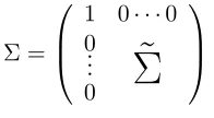
Figure 1: Standardized lengths of various con…dence intervals as function of model size. Dashed lines are added to improve readability.

The standardized lengths of the con…dence intervals corresponding to the constantsKnaive,

K1,. . . ,K5 are reported in Figure 1 for the ten nested submodels mentioned before. We …rst

see that, for each of the constants Knaive, K1, K4, and K5, the standardized length of the

con…dence interval increases with submodel size, which must hold since these constants do not depend on the submodel M and since the term _jjsMjj increases with submodel size (for nested submodels as considered in Figure 1). However, as discussed after Proposition 2.3, the values of K2 and K3 decrease with increasing submodel size for nested submodels. Figure 1

shows that the combined e¤ect of the increase of _jjsMjjand the decrease of K2 and K3 with

obtained fromK2decreases from submodel size6to submodel size8; for the interval obtained

from K3 the standardized length decreases from submodel size 9 to submodel size 10). In

Figure 1 the decreases of the standardized lengths occur only between submodel sizes for which _jjsMjj is almost constant with M (which can be seen from the standardized lengths obtained from, say,K5, since they are proportional tojjsMjj). We also see from Figure 1 that the ‘naive’ interval is much shorter than the other intervals (at the price of typically not having the correct minimal coverage probability). The di¤erence in standardized length between the intervals based onK1 and K2, respectively, is noticeable but not dramatic. A larger increase

in standardized length is noted when comparing the interval based on the costly-to-compute constantK2with the one obtained fromK3, especially for submodel sizes6to9. Furthermore,

the standardized lengths of the con…dence intervals obtained fromK3 are very close to those

obtained from K4 for model size 1 to 9; cf. (18). Finally, in Figure 1 we also see that the

con…dence intervals obtained from K1,K2, and K3 have the same standardized length when

the model size is10, and that the same is true for the con…dence intervals obtained fromK3

and K4 when the model size is 1. This, of course, is not a coincidence, but holds necessarily

as has been noted in the discussion of Proposition 2.3.

Additional computations of con…dence interval lengths, withX andx0now randomly

gen-erated, yield results very similar to those in Figure 1. For the sake of brevity, these results are not shown here. We …nd, in particular, that the standardized length of the con…dence interval obtained fromK3 always increases with submodel size when they are averaged with respect

toX andx0, but, as in Figure 1, can decrease locally when not averaged. [In these additional

numerical studies we did not consider the constant K2 due to the high computational cost

involved in its evaluation.]

4.2 Minimal coverage probabilities

In this section we consider the case where =X and d= p < n, i.e., the case where the given matrixX has full rank less thannand provides a correct linear model for the data Y. We then investigate the minimal coverage probabilities (the minimum being w.r.t. ₂ Rp and ₂(0;₁)) of the intervals obtained from the constants Knaive, K1, K3, and K4 when

used as con…dence intervals for the targetx0₀[ ^M] (_^n)

M on the one hand as well as for the target

x0

0[ ^M] (?)

^

M on the other hand. The constantsK1,K3, andK4are computed based onMequal to the power set of_f1; :::; p_g. We do not report results for con…dence intervals obtained from

K2, since the computation ofK2 is too costly for the study we present below. The results for

con…dence intervals obtained fromK5 would be qualitatively similar to those for con…dence

intervals obtained fromK4, so we do not report them for the sake of brevity.

in computing the constantsKi, i.e., we do not use a restricted universe of models but use M equal to the power set of _f1; :::; p_g. [Additional simulations with no intercept term and no protected explanatory variable lead to results very similar to the ones given in Table 1 below.] Computational details regarding these procedures can be found in Appendix F.

The design matrixXand the vectorx0are generated in the following manner: The10 10

matrix of (uncentered) second moments is chosen to be of the form

=

0 B @

1 0 0 0

~

.. . 0

1 C A;

where we consider three choices for the9 9 matrix ~. For the …rst case, ~ is obtained by removing the …rst row and column of the10 10empirical covariance matrix (standardized by 30 1 = 29) of the variables in the30 10watershed design matrixXRaw. For the second case, we set ~ =Ip~+ (2a+ ~pa2)Ep~withp~= 9,a= 10, and withEp~thep~ p~matrix which has all

entries equal to1. For the third case ~ coincides with the identity matrixIp~, except that the

zero elements in the last row and column ofIp~are replaced by the constantc=

p

0:8=(~p 1) where p~= 9. Similar as in Berk et al. (2013a) and Leeb et al. (2015), we refer to the data set obtained in the second case as the exchangeable data set (as the covariance matrix ~ is permutation-invariant), and to the one obtained in the third case as the equicorrelated data set (as ~ is the correlation matrix of a random vector, the last component of which has the same correlation with all the other components); see Appendix F for more details. For a given con…guration ofnand , we then sample independentlyn+1vectors of dimension10 1such that for each of these vectors the …rst component is1and the remaining nine components are jointly normally distributed with mean zero and covariance matrix ~. The transposes of the …rstnof theses vectors now form the rows of then p design matrixX, while the(n+ 1)-th of these vectors is used for thep-dimensional vectorx0. [It is easy to see that the mechanism

just described generates matrices of full column rank almost surely. The matricesX actually generated were additionally checked to be of full column rank.]

Consider now a given con…guration of n, , the model selection procedure, the target (either the design-dependent or the design-independent target), as well as of a matrixX and a vectorx0that have been obtained in the manner just described. Then we estimate the minimal

(over and ) coverage probabilities (conditional on X and x0) of the con…dence intervals

obtained from the constantsKnaive,K1,K3, andK4 for the given target under investigation.

The minimal coverage probabilities are estimated by a three-step Monte Carlo procedure similar to that of Leeb et al. (2015), which is described in detail in Appendix F. We stress here that the minimal coverage probabilities found by this Monte Carlo procedure are simulation-based results obtained by a stochastic search over a10-dimensional parameter space, and thus only provide approximate upper bounds for the true minimal coverage probabilities.

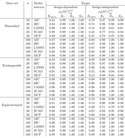
Data set n Model Target

selector design-dependent design-independent

x0[ ^M]0 (_Mn_^) x0[ ^M]0 (_M?_^)

Knaive K1 K3 K4 Knaive K1 K3 K4

Watershed

20 AIC 0.84 0.99 1.00 1.00 0.79 0.97 0.99 0.99 20 BIC 0.84 0.99 1.00 1.00 0.74 0.96 0.98 0.98 20 LASSO 0.90 1.00 1.00 1.00 0.18 0.48 0.61 0.61 20 SCAD 0.90 0.99 1.00 1.00 0.45 0.77 0.84 0.84 20 MCP 0.89 0.99 1.00 1.00 0.47 0.78 0.85 0.85 100 AIC 0.87 0.99 1.00 1.00 0.88 0.99 1.00 1.00 100 BIC 0.88 0.99 1.00 1.00 0.87 0.99 1.00 1.00 100 LASSO 0.88 0.99 1.00 1.00 0.87 0.99 1.00 1.00 100 SCAD 0.88 0.99 1.00 1.00 0.88 0.99 1.00 1.00 100 MCP 0.88 0.99 1.00 1.00 0.88 0.99 1.00 1.00

Exchangeable

20 AIC 0.83 0.99 1.00 1.00 0.80 0.98 0.99 0.99 20 BIC 0.84 0.99 1.00 1.00 0.76 0.97 0.99 0.99 20 LASSO 0.90 1.00 1.00 1.00 0.46 0.86 0.93 0.92 20 SCAD 0.91 1.00 1.00 1.00 0.55 0.90 0.94 0.94 20 MCP 0.91 1.00 1.00 1.00 0.54 0.89 0.94 0.94 100 AIC 0.89 0.99 1.00 1.00 0.90 0.99 1.00 1.00 100 BIC 0.90 0.99 1.00 1.00 0.90 0.99 1.00 1.00 100 LASSO 0.90 0.99 1.00 1.00 0.90 0.99 1.00 1.00 100 SCAD 0.90 0.99 1.00 1.00 0.90 0.99 1.00 1.00 100 MCP 0.90 0.99 1.00 1.00 0.90 0.99 1.00 1.00

Equicorrelated

20 AIC 0.83 0.99 1.00 1.00 0.79 0.98 0.99 0.99 20 BIC 0.81 0.99 1.00 1.00 0.74 0.98 0.99 0.99 20 LASSO 0.88 1.00 1.00 1.00 0.39 0.71 0.79 0.79 20 SCAD 0.88 0.99 1.00 1.00 0.67 0.92 0.95 0.96 20 MCP 0.86 0.99 1.00 1.00 0.66 0.93 0.96 0.96 100 AIC 0.84 0.99 1.00 1.00 0.84 0.99 1.00 1.00 100 BIC 0.86 0.99 1.00 1.00 0.86 0.99 1.00 1.00 100 LASSO 0.88 1.00 1.00 1.00 0.88 1.00 1.00 1.00 100 SCAD 0.88 0.99 1.00 1.00 0.89 1.00 1.00 1.00 100 MCP 0.88 0.99 1.00 1.00 0.89 0.99 1.00 1.00

other intervals in case the LASSO, SCAD, or MCP model selectors are used. However, for

n= 100, these di¤erences are very small for all the con…gurations. This is in line with Lemma C.1 in Appendix C, which entails that for a large family of model selection procedures, the di¤erence of coverage probabilities between the two targets vanishes, uniformly in and , whenn increases. For n= 100, the results are thus almost identical for the two targets: For the …ve model selection procedures, the con…dence intervals obtained from the constantsK1,

K3, andK4 are valid, while the ‘naive’ con…dence intervals are moderately too short, so that

their minimal coverage probabilities are below the nominal level, with a minimum of0:84. Forn= 20and when AIC or BIC is used, the ‘naive’ con…dence intervals fail to have the right coverage probabilities to a somewhat larger extent than in casen= 100. Their minimal coverage probabilities can be as small as 0:81 for the design-dependent target and 0:74 for the design-independent target. [Note that, for the design-dependent target, for n = 20 and

n = 100, the coverage probabilities of the ‘naive’ con…dence interval are generally smaller for the equicorrelated data set than for the exchangeable data set. This can possibly be explained by the fact that Theorems 6.1 and 6.2 in Berk et al. (2013a) suggest thatK1 should

be larger for the equicorrelated data set than for the exchangeable data set. Hence, for the equicorrelated data set, larger con…dence intervals seem to be needed to have the required minimal coverage probability for all model selection procedures.] Furthermore, again for

n= 20 and when AIC or BIC is used, the con…dence intervals obtained from the constants

K1,K3, andK4 remain valid here for both targets.

However, when n = 20 and the LASSO model selector is used, the results for the design-independent target are drastically di¤erent from those obtained with the AIC- or BIC-procedures: All con…dence intervals have minimal coverage probabilities for the design-independent target that are below, and in most cases signi…cantly below, the nominal level. The failure of all the con…dence intervals is here often more pronounced than the failure of the ‘naive’ con…dence intervals when other model selectors are used. Especially for the watershed data set, the estimated minimal coverage probability is0:18 for the ‘naive’ interval and 0:48 for the con…dence interval based on K1. The reason for this phenomenon can be traced to

implementations of these procedures may of course give di¤erent results.

The results in Table 1 concern the coverage probabilities conditional on the design matrix

Xand onx0, and thus depend on the values ofXandx0 used. In additional (non-exhaustive)

simulations we have repeated the above analysis for other values ofX andx0 and have found

similar results.

4.3 Comparison with the con…dence interval of Lee et al. (2016)

In this section we now compare the con…dence intervals of Section 2 with a con…dence interval recently introduced in Lee et al. (2016). Again, we consider the case where = X and

d=p < n, and we focus on the design-dependent target x0

0[ ^M] (n)

^

M . As in Lee et al. (2016) we consider the known-variance case and set = 1 in this section. The con…dence interval of Lee et al. (2016) is dedicated to the LASSO model selector and is given in theR package accompanying that paper for the case wherex0 is a standard basis vector. We hence assume

in the following that x0 is equal to the …rst standard basis vector e1. The proposed interval

is then conditionally valid for the design-dependent target in the following sense: Consider the model selectorM^ obtained by selecting those explanatory variables for which the LASSO estimator has non-zero coe¢cients, with the penalty parameter in (4.1) of Lee et al. (2016) being …xed, independently of Y. Then the interval proposed by Lee et al. (2016), which we denote by CI, satis…es, for any …xed X, for x0 =e1, and for any …xed M f1; :::; pg with

1₂M,

inf

2RpPn; ;1 x

0

0[ ^M] (n)

^

M 2CI M^ =M = 1 ; (21) with the convention that the probability in the above display is1ifPn; ;1( ^M =M) = 0. The

computation ofCI for a given value ofM^ can be carried out without observingx0[ ^Mc], which

is also the case for the con…dence intervals obtained fromK2; :::; K5, but not for that obtained

fromK1. Furthermore, the computation ofCI (when the conditioning additionally is also on

the signs, see Lee et al. (2016) for details) entails a cost that grows linearly with p. Thus,

CI can be implemented for signi…cantly larger values ofp than the con…dence intervals based on K1; :::; K3 currently can be. We note for later use that, in the case x0 = e1 considered

here, the intervalCI as given in Lee et al. (2016) is not de…ned on the event that a model M^

is selected that does not contain1. Hence, we can not speak about unconditional coverage without amending the de…nition in Lee et al. (2016). [A possible amendment, consistent with our conventions and maximizing unconditional coverage among all possible amendments, is to recall that x0₀[ ^M] (n_^)

M = 0 if 1 2= M^ and to set CI = f0g on this event. With such an amendment,CI then a fortiori has minimal unconditional coverage probability not less than 1 .]

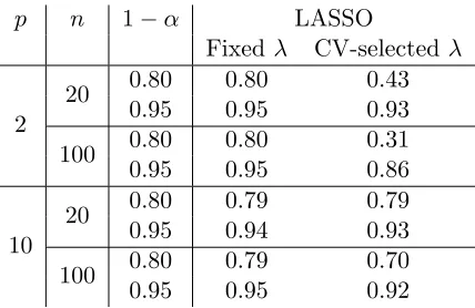
Despite being speci…c to the LASSO model selector with …xed , we nevertheless …nd below that the con…dence interval of Lee et al. (2016) is not shorter than those based on

K1,K3, and K4 (presumably due to the fact that (21) imposes a stricter requirement than