An EnKF based Flow State Estimator for Aerodynamic Problems

(1)

Problems

Thesis by

Andre F. C. da Silva

In Partial Fulfillment of the Requirements for the degree of

Doctor of Philosophy

CALIFORNIA INSTITUTE OF TECHNOLOGY Pasadena, California

2019

(2)

(3)

To my lovely wife. Without her help, sacrifice and encouragement, it simply would’ve never been.

(4)

ACKNOWLEDGEMENTS

First and foremost, I would like to praise God, the author and finisher of all things, for graciously sustaining me at each step of the journey. To Him be honor and glory forever.

I could not have completed this thesis without the guidance, support, encouragement, and counsel of many individuals. Walking alongside me at different stages of the journey, each of them in their own particular way taught me much.

No words can express my admiration to my wife, friend and helper Raquel. Only those close to us know the sacrifices she and my son Daniel had to make so I could pursue this degree, and I am forever grateful for their unwavering love and perennial encouragement. I’m also grateful to my parents for their lifelong support and for teaching me to value of education and pursue excellence. They all have helped to forge who I am today and have made this accomplishment possible.

I own a debt of gratitude to my advisor, Tim Colonius. His unique way of approach-ing problems with curiosity and optimism will always amaze me. I was indeed fortunate to enjoy his mentorship, guidance, and friendship over the last four years. I would also to express my gratitute to my thesis committe (Guillaume Blanquart, Beverley McKeon, and Andrew Stuart) not only for serving in this capacity, but also for the valuable feedback they provided on this thesis. In particular, I am indebted to Andrew for the many meetings in which we discussed the many versions of my estimator. Likewise, I want to acknowledge David Williams and Jeff Eldredge for the many helpful insights provided during the many teleconference meetings we attended.

(5)

I’m also thankful for the care and hospitality of the brothers and sisters from Calvary OPC and Pasadena OPC. Their display of the Christian love truly made the solitude of the last nine months bearable.

Finally, but not least, I’m forever indebted to my extended family and friends back in Brazil and elsewhere. Those are the ones that cheered, prayed and willed me through this doctorate. Every small token of remembrance and affection were of extreme importance for me.

(6)

ABSTRACT

Regardless of the plant model, robust flow estimation based on limited measure-ments remains a major challenge in successful flow control applications. Aiming to combine the robustness of a high-dimensional representation of the dynamics with the cost efficiency of a low-order approximation of the state covariance matrix, a flow state estimator based on the Ensemble Kalman Filter (EnKF) is applied to two-dimensional flow past a cylinder and an airfoil at high angle of attack and low Reynolds number. For development purposes, we use the numerical algorithm as both the estimator and as a surrogate for the measurements. In a perfect-model framework, a reduced number of either pressure sensors on the surface of the body or sparsely placed velocity probes in the wake are sufficient to accurately estimate the instantaneous flow state. Because the dynamics of these flows are restricted to a low-dimensional manifold of the state space, a small ensemble size is sufficient to yield the correct asymptotic behavior. The relative importance of each sensor location is evaluated by analyzing how they influence the estimated flow field, and optimal locations for pressure sensors are determined.

(7)

(8)

PUBLISHED CONTENT AND CONTRIBUTIONS

[1] D. Darakananda et al. “EnKF-based Dynamic Estimation of Separated Flows with a Low-Order Vortex Model”. In:2018 AIAA Aerospace Sciences Meet-ing. AIAA 2018-0811. Reston, Virginia: American Institute of Aeronautics and Astronautics, Jan. 2018. doi:10.2514/6.2018-0811.

A.F.C.S. participated in the conception and implementation of the estimator, and participated in interpretation of the results.

[2] A. F. C. da Silva and T. Colonius. “A Bias-aware EnKF Estimator for Aerodynamic Flows”. In: 48th AIAA Fluid Dynamics Conference. AIAA 2018-3225. Reston, Virginia: American Institute of Aeronautics and Astro-nautics, June 2018. doi:10.2514/6.2018-3225.

A.F.C.S. participated in the conception and implementation of the estimator, obtained the simulation data, and was the principle author of the manuscript. [3] A. F. C. da Silva and T. Colonius. “Ensemble-Based State Estimator for Aerodynamic Flows”. In: AIAA Journal (June 2018), pp. 1–11. doi: 10. 2514/1.J056743.

A.F.C.S. participated in the conception and implementation of the estimator, obtained the simulation data, and was the principle author of the manuscript. [4] X. An et al. “Response of the Separated Flow over an Airfoil to a Short-Time Actuator Burst”. In: 47th AIAA Fluid Dynamics Conference. AIAA 2017-3315. Reston, Virginia: American Institute of Aeronautics and Astronautics, June 2017. doi:10.2514/6.2017-3315.

A.F.C.S. participated in the conception of the project, and participated in interpretation of the results.

[5] A. F. C. da Silva and T. Colonius. “An EnKF-based Flow State Estimator for Aerodynamic Flows”. In: 8th AIAA Theoretical Fluid Mechanics Confer-ence. AIAA 2017-3483. Reston, Virginia: American Institute of Aeronautics and Astronautics, June 2017. doi:10.2514/6.2017-3483.

(9)

LIST OF ILLUSTRATIONS

Number Page

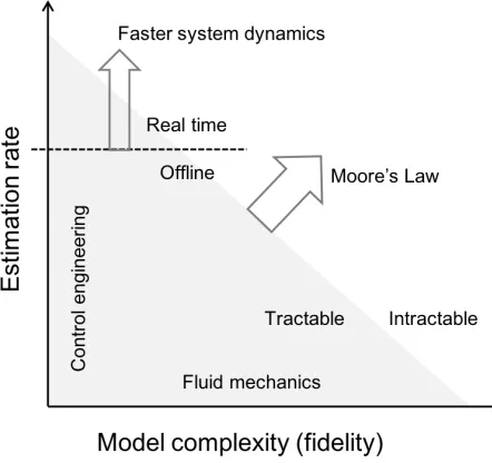
1.1 Schematics on the current development of estimation techniques in the fluid mechanics context. . . 2 1.2 Graphical representation of the estimation process. Reproduced from

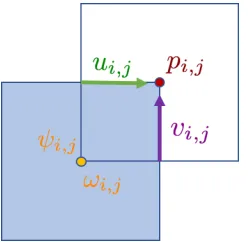
[37] with permission. . . 15 1.3 Schematic representation of the EnKF algorithm. . . 24 2.1 Variables placement on a staggered grid with respective dual mesh. . 42 2.2 Comparison between different choices of the discrete delta function. . 43 2.3 Contour plot of the computed pressure coefficient field, overlapped

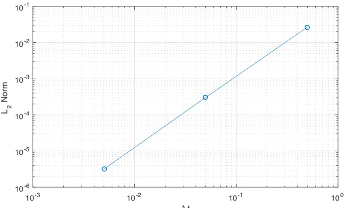
with isocurves of vorticity. . . 46 2.4 Convergence plot for the semi-discrete force update. . . 47 2.5 Low-rank behavior of the low-Re incompressible flow past inclined

flat plate and airfoil (NACA 0012). . . 49 2.6 Vorticity contours for the flow past a circular cylinder atRe =100. . 50 2.7 Flow past a circular cylinder: location of the velocity measurement

points in the flowfield. . . 51 2.8 Location of the pressure measurement points over the surface of a

NACA 0009 airfoil. . . 51 2.9 Vorticity contours for the the flow past a NACA 0009 airfoil atAoA=

30 deg and Re= 200. . . 52 2.10 Vorticity contours for the flow past a flat plate at AoA = 30 deg and

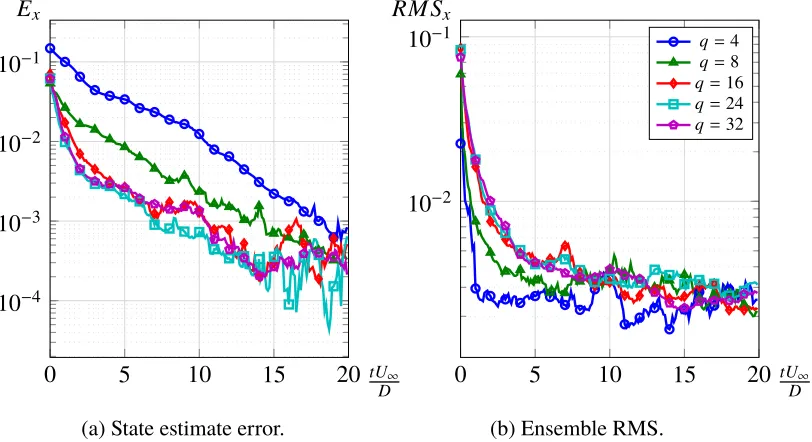
Re =200. . . 52 3.1 Effect of the choice of the initial ensemble on the estimator performance. 56 3.2 Estimator performance for increasing ensemble sizes applied to the

problem of the flow past a circular cylinder atRe =100 using velocity measurements. Measurement error level is set to R= 10−4Ip. . . 56

(13)

3.4 Measurement influence fields (representers) for the horizontal com-ponent of the fluid velocity at selected measurement locations. En-semble size was 16 members and R = 10−4Ip. All the figures have

the same contour levels. . . 59 3.5 Estimated lift coefficient evolution using the RTPS covariance

infla-tion scheme (θ =0.95). . . 60 3.6 Estimator performance for different multiplicative covariance

infla-tion schemes applied to the flow past a NACA 0009 at high angle of attack. Ensemble size is 24 and the sensor noise level is set toR=10−4. 61 3.7 Histograms used in the iterative process of finding the optimal

pres-sure sensor placement. . . 62 3.8 Estimated and reference vorticity field 20 convective time units

af-ter estimator initialization using a single pressure sensor optimally placed near the leading edge. . . 63 3.9 Time spent in each of the filtering steps for the EnKF simulation

with pressure measurements, implicit linearization scheme, and q = 60. Twelve threads were used to split the computational load in the forecast step and when gathering measurements. . . 65 3.10 Effect of nonlinear observation model in the estimator performance in

the perfect-model framework. Solid lines correspond to the iterative (Gauss-Newton) method and dashed lines, to the implicit lineariza-tion scheme. . . 66 3.11 Examples of the sample autocorrelation function for different

mea-surement locations. Horizontal dashed lines correspond to the asso-ciated upper and lower confidence bounds, respectively. . . 68 3.12 Optimality of the EnKF with pressure measurements as perceived

from the decay of the innovation autocorrelation function. Mea-surement points are numbered from the leading edge to the trailing edge. . . 70 3.13 Optimality of the EnKF with velocity measurements as perceived

from the decay of the innovation autocorrelation function. Measure-ment points are numbered from left to right, and from the bottom to the top. . . 71 3.14 Optimality of the EnKF with pressure measurements as perceived by

(14)

3.15 AR order attributed by the second test to each of the pressure mea-surement points. . . 73 3.16 Optimality of the EnKF with velocity measurements as perceived by

finding the best AR model that represents the innovation sequence. . 73 3.17 AR order attributed by the second test to each of the velocity

mea-surement points. First and second values correspond, respectively, to the horizontal and vertical component of the velocity vector. . . 74 3.18 3D-EnVar estimator performance for different values ofαapplied to

the problem of the flow past a flat plate at Re = 200 and AoA= 30° using velocity measurements. Measurement error level is set to R= 10−4Ip. . . 75

4.1 Estimated lift coefficient for airfoil with randomized freestream ve-locity using the RTPS covariance inflation scheme. . . 79 4.2 Estimated lift coefficient for decelerating airfoil (75% of its initial

velocity over 13.3 convective time units) using the RTPS covariance inflation scheme. . . 80 4.3 Joint parameter/state estimation for an airfoil decelerating to 75% of

its initial value over 13.3 convective time units. The measurement noise level is set to R= 10−6Ip. . . 81

4.4 Estimated lift coefficient for decelerating airfoil (75% of its initial velocity over 1 convective time units) using the RTPS covariance inflation scheme. . . 82 4.5 Estimated lift coefficient for decelerating airfoil (75% of its initial

velocity over 1 convective time units) using the RTPS covariance inflation scheme and explicit stochastic forcing. . . 82 4.6 Evolution of the estimated parameters covariance for an airfoil

decel-erating to 75% of its initial value over one convective time unit. The measurement noise level is set to R= 10−6Ipand the RTPS inflation

level is set to θ = 0.90. The dashed line ( ) corresponds to the unforced simulation and the solid line ( ) represents the estima-tion dynamics with the explicit stochastic forcing in the perturbaestima-tion derivative dynamics (noise covariance level 10−8). . . 83 4.7 Joint parameter/state estimation for an airfoil decelerating to 75%

(15)

4.8 Error in the estimation of the freestream parameters for an airfoil decelerating to 75% of its initial value over one convective time unit. The measurement noise level is set to R = 10−6Ip and the RTPS

inflation level is set toθ =0.90. In both plots the error is normalized by the maximum perturbation in the interval. . . 84 4.9 Estimated lift coefficient for an airfoil subjected to random freestream

perturbation. . . 85 4.10 Joint parameter/state estimation for an airfoil subjected to random

freestream perturbations (reduced cutoff frequency is two). The mea-surement noise level is set toR=10−6Ipand the RTPS inflation level

is set to θ = 0.90. The dashed line ( ) corresponds to the actual perturbation, and the solid line ( ) represent the estimated val-ues with the explicit stochastic forcing in the perturbation derivative dynamics (magnitude 10−8). . . 85 4.11 Estimated Re for the flow past an inclined flat plate using pressure

measuremerts and the RTPS covariance inflation scheme (θ = 0.9 and R=10−4Ip). . . 86

5.1 Sources of bias in an Kalman-based estimator. . . 89 5.2 Temporal average of the bias fields introduced by the resolution error

for the flow past an inclined flat plate when comparing the Re∆ = 1 (200 grid points per chord) simulation to the correspondingRe∆ =4 (50 grid points per chord) simulation. . . 99 5.3 Temporal average of the bias fields introduced by the resolution error

for the flow past an inclined NACA 0009 when comparing theRe∆ =1 (200 grid points per chord) simulation to the correspondingRe∆ =4 (50 grid points per chord) simulation. . . 100 5.4 Fraction of the bias variance left out by using the corresponding first

POD modes for the flow past an inclined flat plate and a NACA 0009 airfoil. . . 101 5.5 Prediction error corresponding to the best (in a least-squares sense)

ARn model for each of the POD modes selected to represent the bias. The order of the corresponding auto-regressive model increases from 1 to 10 as the color of the curves changes from dark to light. . . 102 5.6 Ritz values corresponding to the DMD modes of the bias (when a

(16)

5.7 Prediction error corresponding to DMD-based low-rank models with different number of DMD modes. . . 103 5.8 Illustration of the different domains used for the evaluation of the

state error. The small circles on the surface of the plate represent the locations where the pressure measurements are taken. . . 104 5.9 Bias-blind estimator performance highlighting the deleterious effect

of the dynamics and observation bias (R= 10−4). Black lines corre-spond to the mean square error evaluated in the entire computational domain, while the gray lines restrict this evaluation to the region outside an unit circle centered at the plate. . . 105 5.10 Bias-aware estimator performance (R = 10−4, λo =

√

10/10 and

λs = √10/10). Black lines correspond to the mean square error evaluated in the entire computational domain, while the gray lines restrict this evaluation to the region outside a unit circle centered at the plate. . . 106 5.11 Effect of the magnitude of the process noise to bias dynamics (R =

10−4). Solid lines correspond to the mean square error evaluated in the entire computational domain, while dashed lines restrict this evaluation to the region outside an unit circle centered at the plate. . . 107 5.12 Estimated pressure on the surface of the flat plate at end of a

simula-tion window (tU∞/c= 20). . . 108

5.13 Bias-aware estimator performance with imperfect statistics (R = 10−4). Solid lines correspond to the mean square error evaluated in the entire computational domain, while the dashed lines restrict this evaluation to the region outside a unit circle centered at the plate. 109 5.14 Effect of different choices of models for the bias dynamics on the

performance of the bias-aware estimator. Solid lines correspond to the mean square error evaluated in the entire computational domain, while the dashed lines restrict this evaluation to the region outside a unit circle centered at the plate. . . 109 5.15 Bias-aware estimator performance (R= 10−4,λo=1/10 andλs =1)

(17)

5.16 Estimated pressure on the surface of the NACA 0009 at the end of a simulation window (tU∞/c= 30). . . 111

B.1 Comparison of the lattice Green’s function to its continuous counter-part for h=1. . . 127 B.2 LGF-based solution corrected to account for the offset. Left axis

(18)

LIST OF TABLES

Number Page

1.1 Summary of the recent contributions to the area of flow estimation. . 6 3.1 Norm of the mean normalized innovation for different choices of

(19)

NOMENCLATURE

α. multiplicative covariance inflation parameter.

β. additive covariance inflation parameter.

Γx,Γy. respectively, dynamics and observation bias low-rank models.

1. 1-dimensional vector of ones.

E[·]. expectation operator defined in Eq. 1.3.

µk, νk. process (i.i.d. N(0,Q)) and observation (i.i.d. N(0,R)) noises.

ρ(·). probability density function.

ξk, ηk. respectively, dynamics and observation bias parameters. Ak. state perturbation matrix (see Eq. 5.16) at timetk.

c. dimension of the control vector.

C_kxy. cross-covariance matrix between variables x andyat timetk.

Ex,Ey. state and observation estimate errors, respectively. f :_Rn 7→_Rn. (possibly nonlinear) dynamic model. h:Rn7→ Rp. (possibly nonlinear) observation model.

M(τ). autocorrelation matrix with lagτ. n. dimension of the system state vector.

no. dimension of the observation bias parameters vector.

ns. dimension of the state bias parameters vector.

p. dimension of the measurement/observation vector. q. ensemble size.

Re. Reynolds number U∞_νL, whereL is a reference length.

RM Sx,RM Sy. state and observation ensemble root mean square errors, respectively.

vk. analysis correction coefficients.

xk. system state vector at timetk.

yk. vector of measured quantities at timetk.

Zk. state ensemble matrix (each column represents the state of the corresponding

(20)

C h a p t e r 1

INTRODUCTION

1.1 Motivation

In the aeronautical context, unsteady conditions, such as the ones that would result from a maneuver or from the occurrence of gusts, are ever present. The agility and maneuverability of a fighter or the perceived level of comfort of a commercial aircraft could be significantly enhanced if we could robustly estimate the instantaneous flow state from the available measurement data (e.g. pressure readings on the wings and fuselage), and act accordingly using closed-loop flow control[1]. In this work we focus on one of the two key ingredients to any successful closed-loop control design: the ability to predict the state of a fluid system and forecast its evolution.

Figure 1.1 can be used to describe how different scientific communities have been approaching the dilemma between model complexity (x-axis) and estimation rate (y-axis). Estimation rate refers to the number of forecasts per unit time, and, for on-line estimation, is set by the system’s dynamics but highly constrained by the available computational power. The gray area between the axis represents the choices of model complexity and estimation rate that are achievable with the currently available computational power. The horizontal dashed line represents the minimum estimation rate that would allow us real-time prediction. Because standard estimation techniques don’t scale well with an increasing number of degrees of freedom, the control engineering community will generally favor low-rank models that preserve limited, but dynamically important, features of the system. On the other hand, fluid mechanicists, particularly those in the CFD community, typically use every addition to the available computational power to simulate models that are more complex and reliable than their predecessors, even if these simulations take months.

(21)

[image:21.612.174.395.177.385.2]

can be made small enough to allow the use of the standard algorithms, but their well-known fragility to the specification of initial conditions and flow parameters (e.g., Reynolds number) can constitute a major applicability limitation. Therefore, it would be desirable to seek more robust solutions that lie close to the intersection of the real-time barrier with the computational power barrier.

Figure 1.1: Schematics on the current development of estimation techniques in the fluid mechanics context.

(22)

1.2 Bibliographic Review

Table 1.1 summarizes recent works on data-driven flow estimation. Two main goals have driven the fluid mechanics community to combine numerical models and experimental data: flow reconstruction and flow prediction.

The first application is as a form of extending the experimental reach by performing what is commonly referred to as enhanced experiment or hybrid simulation. As pointed out by Nisugi, Hayase, and Shirai [6], taken individually, computational fluid dynamics (CFD) and experimental data lack the ability to fully represent the physical phenomena under scrutiny. Despite being a direct observation of the true physics, experimental data is inevitably corrupted by noise and only a small subset of the relevant physical information can be measured1. In addition, there can be uncertainties and biases in the transduction process. On the other hand, limited computational resources restrict our ability to accurately represent the underlying flow physics, especially for higher Reynolds numbers. Moreover, assumptions regarding the initial and boundary conditions are often too simplistic to accurately represent the conditions that would be encountered in an experimental setting. But, despite all these limitations, a numerical solution allows for the evaluation of physical quantities that are unattainable using instrumentation. By combining the strengths of both approaches, the resulting hybrid solution is able to provide flow information that is consistent with the observed experimental data and recovers quantities that were not directly observed in the experiment Hayase [7].

Nisugi et al. [6] and Hayase et al. [5] incorporated measurement data into a simulation using a feedback controller whose constant gain was determined by trial and error to obtain the best fit to experimental data. Other researchers formulated this problem from a variational perspective, in which they seek to minimize a cost functional describing the data mismatch subjected to constraints2[8]. Papadakis and Memin [9] and Gronskis, Heitz, and Memin [10] treated the system dynamics as deterministic, and used a variational framework to estimate the initial and boundary conditions that were most consistent with the available observations.

Suzuki et al. [11, 12] examined the problem of estimating the flow past a NACA 0012 airfoil for different angles of attack and Re between 103 and 104. Their

1_{This limitation can manifest itself in many ways: limited field of view, limited temporal and}

spatial resolution, methodological inability to measure some quantities (e.g., vorticity or Reynolds stresses), etc.

2_{The constraints can be dynamical, such as enforcing the estimate to be a solution of the}

(23)

assimilation approach consisted in taking a weighted averaged of the DNS solution and a rectified version of the experimental data. The rectification procedure ensured that the added data satisfied the divergence-free condition. Their conclusion was that the hybrid simulation performed better3 than an unsteady Reynolds-averaged Navier-Stokes (URANS) simulation for higher angles of attack. Foures et al. [13] and Symon et al. [14] used a variational method to incorporate observations of the mean velocity profile into a RANS simulation in order to reduce the amount of measurement noise and estimate physical quantities, such as the Reynolds shear stress, that were not directly measured.

The second goal of data assimilation has closed-loop control in mind. In this case, the estimator accuracy requirements must be weighed against turnaround time (see Fig. 1.1). Within the flow control community, the most common approach to flow estimation is the development of reduced-order models (ROMs) whose number of degrees of freedom are small enough to be tractable with the classical estimation techniques. Provided these models have a low number of degrees of freedom, then the classical control techniques become feasible. Gerhard et al. [15] used a 3-mode POD-Galerkin model (enhanced with the shift mode) to design a controller to suppress vortex shedding behind circular cylinders at low Reynolds numbers. Aleksic et al. [16] used data from 15 pressure sensors and a 5-mode Galerkin model to decrease and stabilize the drag of a 2D bluff body. Ahuja and Rowley [2] used a 22-mode ROM obtained by Balanced Truncation to design a LQG controller for the flow past an inclined flat plate. Flinois and Morgans [3] used the Eigenvalue Realization Algorithm (ERA) to construct an unstable 10-mode ROM which was then used to designH∞controllers to stabilize the system. These ROMs, however,

are fragile with respect to initial conditions and flow parameters like the Reynolds number[1]. Alternatively, researchers such as Fukumori and Malanotte-Rizzoli [17] and Suzuki [18] proposed the use of reduced-order approximations to the Kalman filter that restrict the correction to the larger scales of the solution and alleviate the computational cost involved.

As an alternative approach, researchers in fields such as meteorology, oceanography and geophysical fluid dynamics have developed data assimilation algorithms that are inherently capable of dealing with high-dimensional nonlinear systems and high volumes of measurement data [19, 20]. These methods take advantage of the increasingly available computational power and efficient parallel implementations,

3_{The hybrid simulation produced better estimates for the lift coefficient and the dynamics of the}

(24)

and had not, until recently, received much attention from the flow control community. A three-paper series by Bewley and his collaborators aimed to apply Kalman filtering to devise a state estimator for laminar [21] and turbulent channel flow[22, 23]. Following a rigorous derivation of stochastic models for the system noises, they were able to successfully track the wall-normal velocity and vorticity based on pressure and wall skin friction. For the turbulent channel flows, an Ensemble Kalman Filter was shown to achieve at least one order of magnitude less error than previously reported in the literature at 20 viscous units from the wall. Around the same time, Kato and Obayashi [24] used the Ensemble Kalman Filter to estimate the velocity field behind a square cylinder by assimilation of pressure measurements at the faces of the body. These two papers appear to be the first application of ensemble-based estimation methods to classical fluid dynamics problems.

Recent applications of the EnKF include Kikuchi, Misaka, and Obayashi [25], who compared the performance of a EnKF and a Particle Filter applied to a POD-Galerkin model of the problem of the flow past a cylinder, and Kato et al. [26], who used a variation of the EnKF to achieve synchronization between a RANS numerical simu-lation of a steady transonic flow past airfoils and pressure experimental data. Mons et al. [27] used an ensemble Kalman smoother and other ensemble-based variational methods to reconstruct freestream perturbation history based on measurements taken on and around a circular cylinder subjected to it.

(25)

6

Estimated Flow

Reference IP/DA4 Methodology Description Re5 Estimated

Quantities

Estimator

Model Measurements

Bewley and Protas [28] DA Adjoint Incompressible 3D

turbulent channel flow 100 Initial State

Linearized

N-S

Skin friction and

pressure

distribution

Hayase, Nisugi, and

Shirai [5] and Nisugi,

Hayase, and Shirai [6]

DA Constant-gain observer

Flow past a square

cylinder 1200 Velocity field DNS

Pressure on square

faces

Hoepffner et al. [21] DA KF/EKF 3D Laminar channel flow 3000

Wall-normal

velocity and

vorticity

Linearized

N-S

Skin friction and

pressure

distribution

Chevalier et al. [22] DA EKF 3D Turbulent channel

flow 100

Wall-normal

velocity and

vorticity

Linearized

N-S

Skin friction and

pressure

distribution

Ruhnau, Stahl, and

Schnorr [29] DA Adjoint Synthetic turbulent flow 10 Vorticity field DNS Optical flow

Papadakis and Memin [9] DA Adjoint Incompressible 2D turbulent field

Not

re-ported

Initial State DNS Velocity field

[image:25.612.71.740.135.478.2]

(26)

7

Estimated Flow

Reference IP/DA Methodology Description Re Estimated Quantities

Estimator

Model Measurements

Suzuki, Ji, and

Yamamoto [11] and

Suzuki et al. [12]

DA Weighted

average Flow past a NACA 0012

103−

104 Velocity field DNS TR-PTV

Colburn, Cessna, and

Bewley [23] DA EnKF

3D Turbulent channel

flow 100

Wall-normal

velocity and

vorticity

DNS

Skin friction and

pressure

distribution

Kato and Obayashi [24] DA EnKF Flow past a square

cylinder 1200 Velocity field DNS

Pressure on square

faces

Suzuki [18] DA Low-rank

Approx. EKF Planar jet flow 2000 Velocity field DNS TR-PTV

Gronskis, Heitz, and

Memin [10] DA Adjoint

Flow past a circular

cylinder 172

Boundary and

initial conditions DNS Vorticity field

Foures et al. [13] IP Adjoint Flow past a circular

cylinder 150

Reynolds stress

tensor RANS Velocity field

Kato et al. [26] IP EnKF Transonic flow past an airfoil and a wing

106−

107

Flow variables +

turbulent viscosity RANS cpon surfaces

[image:26.612.78.742.127.451.2]

(27)

8

Estimated Flow

Reference IP/DA Methodology Description Re Estimated Quantities

Estimator

Model Measurements

Kikuchi, Misaka, and

Obayashi [25] DA EnKF/PF

Flow past a circular

cylinder 1000 ROM coeffs

POD-Galerkin

ROM

Velocity in the

wake

Mons et al. [27] DA EnKS/4DVar/ 4DEnVar

Circular cylinder

subjected to gusts 100

Boundary and

initial conditions DNS

cp,CD,CL and

velocity field

Mons, Chassaing, and

Sagaut [30] DA Adjoint Rotating cylinder 100 Initial State andΩ DNS

CD,CL, and

velocity field

Meldi and Poux [31] DA

Filtered-Covariance

KF

Circular Cylinder/Thick

Plate

100/

80000

Velocity and

pressure field DNS/DDES Velocity field

Symon et al. [14] and

Symon [32] IP Adjoint Flow past an airfoil 13500

Reynolds stress

tensor RANS Velocity field

Darakananda et al. [33] DA EnKF Inclined flat plate 500 Vortices strengths and positions

Aggregated

vortex

model

Pressure on the

surface

Present Study[34, 35] DA EnKF

Incompressible 2D flow

past a cylinder, a flat plate

or an airfoil

100/200

Vorticity field and

additional

parameters

Unresolved

DNS + Bias

modeling

Velocity in the

wake or pressure

[image:27.612.74.739.127.481.2]

(28)

1.3 Mathematical Background

By the very nature of an estimation problem, the state x ∈ _Rn of any dynamical system6 is only knowable up to a certain level of uncertainty. Mathematically, this behavior is represented by a random vector whose possible values correspond to individual realizations of the underlying random process. The probability that its value falls in any given subsetA∈_Rn_{of the state space is given by}

P(x ∈ A)=

∫

A

ρ(x)dx , (1.1)

where the probability density function (PDF) ρ:Rn7→ R+satisfies

∫

Rn

ρ(x)dx =1 . (1.2)

For any function f of the state, we define the corresponding expected value by

E[f(x)]=

∫

Rn

f(x)ρ(x)dx. (1.3)

When it is necessary to make explicit which PDF the expectation refers to, the notation_Eρ[·]will be used.

An alternative way of describing the PDF of a random variable is through a sequence of central momentsαigiven by

αi =    ¯

x =E[x] i=1 diMx

dti

t=0 i>1 ,

(1.4)

whereMx(t)= E[exp(tT(x−x))]¯ 7is the corresponding moment-generating function.

In particular, note that the first-order momentα1 = x¯ corresponds to the mean of the distribution, and the second-order central moment α2 correspond to the auto-covariance matrix Cx x. According to the inverse theorem, if Mx(t)is finite for all

t ∈ {x ∈_R| kxk < a} for somea > 0, thenMx(t)uniquely determines the PDF of

x. Therefore, in order to track the time evolution of the state of a system, one needs to predict how the PDF changes over time, either directly or indirectly (by tracking its moments).

4_{IP stands for Inverse Problem, and DA stands for Data Assimilation. The latter differs from the}

former by assuming a temporal evolution of the variable being tracked.

5_{This quantity is defined differently for each problem.}

6_{Despite the fact that the dynamics of fluid systems are inherently infinite-dimensional, we}

employ a discretization scheme to produce a finite-dimensional approximation suitable to be used in a computed simulation.

7_{Note that variable}_t_{here has the same dimension as}_x_{, so that}_M

(29)

Besides the mean, another important feature of the PDF is the mode. The mode rep-resents the most likely value of the corresponding random variable. Mathematically, it is given by

mx =arg max

x∈_Rnρ(x). (1.5)

Note that the mode need not to be unique and secondary modes corresponding to local maxima may be present.

1.3.1 Weighted Inner Product and Norm

For an ordered pairu,v ∈_Rn, we denote the corresponding Euclidean inner product as

hu,vi = uTv (1.6)

and its induced L2-norm as

kuk2= hu,ui ≥0 , (1.7)

where the equality holds if, and only if,u= 0.

For any positive-definite symmetric matrixA, the A-induced weighted norm is given by

kukA = kA−1/2uk. (1.8)

1.3.2 Gaussian Random Variables

A Gaussian8 random variable (GRV) on Rn is characterized by its mean ¯x ∈ Rn

and a positive-semidefinite covariance matrix C ∈ _Rn×n, and is often denoted as x ∼ N(x¯,C). Its associated PDF is given by

ρ(x)= 1

(2π)n/2₍_det_C₎1/2exp

−1

2 kx−x¯k 2

C

. (1.9)

The matrixC−1/2is often called the precision matrix of the Gaussian random vari-able. Note also that for a GRV, the mean and mode of the distribution coincide. Gaussian-distributed random variables can be completely represented by their mean and variance, linear combination of GRVs are also Gaussian-distributed, and apply-ing linear operators to such variables will always result in new Gaussian-distributed random variables.

(30)

1.3.3 Conditional Distributions

If(x,y) ∈_Rn×pis a jointly varying random variable, the conditional PDF ρ(x|y)is defined as

ρ(x|y)= ρ(x,y)

ρ(y) , (1.10)

whereρ(y)corresponds to the marginal PDF of ygiven by

ρ(y)= ∫

Rn

ρ(x,y)dx. (1.11)

1.3.4 Bayes’ Theorem

Bayes’ theorem states that for a jointly varying random variable(x,y) ∈_Rn×p

ρ(x|y)= ρ(y|x)ρ(x)

ρ(y) . (1.12)

This theorem is one of the cornerstones of the Bayesian inference, and expresses how prior beliefs (ρ(x)) should be updated to account for new evidence (ρ(y)) assuming a model that describes the likelihood of obtaining determined data given that the state (ρ(y|x)) is known. The resulting distribution (ρ(x|y)) is often referred to as the posterior.

1.3.5 Maximum a Posteriori vs Minimum Variance Estimates

An estimator ˜x(y) is a function of the observation y ∈ _Rp that aims to provide the best estimate of x according to some criteria. In the Bayesian context, a first important notion of optimality is the minimization of the mean square error (MSE), given by the trace of the error covariance matrix

M SE(x˜)= trE[(x˜−x)(x˜−x)T] =E[(x˜−x)T(x˜− x)]. (1.13)

The minimum-MSE estimator is then defined as the function

˜

xM M SE(y)= arg min

˜

x:Rp7→Rn

M SE(x)˜ . (1.14)

It can be shown [36] that as long as the underlying PDF admits finite mean and covariance matrix, the minimum variance estimate is the conditional mean

˜

(31)

A second possible optimality criteria is carried out by the maximum a posteriori (MAP) estimator. It is defined as the mode of the posterior distribution obtained by applying Bayes’ theorem.

˜

xM AP(y)=arg max

˜

x:Rp7→Rn

ρ(x˜|y)=arg max ˜

x:Rp7→Rn

ρ(y|x˜)ρ(x˜)

ρ(y) =arg max

˜

x:Rp7→Rn

ρ(y|x˜)ρ(x˜). (1.16)

Note that when the posterior is Gaussian, the MMSE and the MAP estimator are equivalent since the mode and the mean of a Gaussian coincide.

A third criteria would be the maximum likelihood (ML) estimator. Here ˜x(y) is defined as the state that is more likely to produce the observed y, regardless of any a priori information on x. In other words,

˜

xM L(y)=arg max

˜

x:Rp7→Rn

ρ(y|x)˜ . (1.17)

Note that the ML and MAP estimators coincide when the prior is a uniform distri-bution.

MMSE estimators are global in the sense that they summarize the information contained in the whole PDF when evaluating the conditional mean. On the other hand, MAP estimators only highlight local features of the posterior PDF, something that can be troublesome if the posterior is multi-modal, for instance.

1.3.6 Dynamical Systems

A general discrete-time controlled dynamical system can be characterized by a se-quence of functions fk ∈C(Rn×Rc,Rn), often referred to as the forecast model, that

describe the time evolution of the state of the system subjected to some control input. These functions represent the available deterministic knowledge about the system at hand. When nondeterministic or unmodeled aspects of the underlying physical phe-nomenon are present, their effect can be taken into account stochastically. Consider the stochastic dynamical system

xk+1= fk(xk,uk)+ µk , (1.18)

where fk is a general function of then-dimensional state xk, uk is ac-dimensional

control input vector, and µkis an i.i.d. sequence with PDF ρsthat accounts for state disturbances and process noises. The subscript k refers to quantities taken at time t =tk. The trajectory of this system corresponds to a Markov chain for which

(32)

so that the probability that xk+1 ∈S ⊂ Rnis given by

P(xk+1 ∈S|xk)=

∫

S

ρs(x− fk(xk,uk))dx. (1.20)

We also assume that system is at least partially observable, and that there is a function h ∈ C1(_Rn_,

Rp) that maps the state to any observable quantity. Since in

any realistic measurement methodology involves uncertainties (noise), the typical observation model will take the form

yk = h(xk)+νk . (1.21)

whereh(x)is the observation function (yk is a p-dimensional vector), andνk is an

i.i.d. sequence with PDF ρothat represents the sensor noise. Thus,

ρ(yk|xk)= ρo(yk −h(xk)), (1.22)

so that the probability that yk ∈S ⊂ Rpis given by

P(yk ∈S|xk)=

∫

S

ρo(y−h(xk))dx. (1.23)

1.4 Data Assimilation

Given a dynamical system, there are two ways of estimating its current state. A first one requires knowledge of the state at previous times, and a forecast model that describes the time evolution of the system. Combined, they can be used to estimate the trajectory of the system. The accuracy of theses predictions, however, relies not only on the preciseness of our estimate of the initial conditions but also on the reliability of the model itself. The fidelity of the chosen model is limited not only by our understanding of the dynamics of the system, but also by how fast are we expected to produce such estimate given computational resources.

(33)

Given these two estimates for the state of the system, one predicted from inaccurate previous estimates and another inferred from limited available data, the goal of the data assimilation is to determine the optimal strategy of managing the available re-sources and combining them in order to produce an estimate that meets the accuracy requirements.

DA methods can be classified as variational and sequential. The goal of variational methods is to optimize the estimated trajectory of the system over a given time inter-val while fulfilling model dynamics and conforming to the available measurements. The problem formulation involves the definition of a cost function (which penal-izes the mismatch between predicted and measured data and enforces the system dynamics) in terms of a control variable (e.g., initial state). The evaluation of the optimal control variable typically involves iteration and derivatives in the form of a sensitivity, or adjoint, model. On the other hand, sequential methods get their name from the fact that they are usually formulated as a sequential repetition of two basic steps: when new measurements are available, corrections are applied to the state estimate (analysis step); then, the state statistics are propagated forward in time using the available dynamic model (forecast step) until new measurements become available again. Figure 1.2 shows a graphical representation of a sequential estimation process. The points and oval regions represent, respectively, the mean and uncertainty (which can be seen as a contour level of the underlaying PDF) of each estimate. Estimation methodology combines model prediction (blue figure) to the state inferred from the measurements (red figure) to yield an improved state estimate (green figure).

Algorithmically speaking, sequential methods are more flexible with respect to the choice of forecast models. Because they do not require the corresponding linearized forward and adjoint operators, models can be treated as black boxes. In terms of performance, sequential methods tend to favor the use of more complex models in real-time applications, since a single forward integration is needed.

(34)

[image:34.612.211.402.74.268.2]

Figure 1.2: Graphical representation of the estimation process. Reproduced from [37] with permission.

1.4.1 Kalman Filtering

The fundamentals of optimal filtering9were laid down by Kalman [4]. The classical Kalman filter provides a rigorous solution for the state estimation of linear systems under Gaussian-distributed noise. The goal of Kalman filtering is to use measure-ment data to construct an estimate of the statexkwhich is optimal in the sense that it

minimizes the estimation variance (or, equivalently, maximizes the likelihood) [41]. The estimate is regarded as a Gaussian-distributed random variable which is charac-terized by its meanxk and covarianceCk. Assuming linearity, fk(x,u)=Fkx+Bku

andh(x)= H xEq. 1.18 and 1.21 can be rewritten as

xk+1 = Fkxk+Bkuk+ µk (1.24a)

yk = Hkxk+νk . (1.24b)

We also assume both µk and νk are zero-mean, Gaussian, and white random pro-cesses (µk ∼ N(0,Qk)andνk ∼ N(0,Rk)) that are uncorrelated in time (E[µkµT_l]=

Qkδkl andE[νkν_lT]= Rkδkl, whereδkl is the Kronecker delta)10.

DefiningYk = {y1 y2 · · · yk} as the set that collects all the measurements taken

from the system up to timet = tk, it can be shown that the optimum filtering process

for the unforced system (u= 0) can be synthesized in two steps [42]:

9_{In this context, filtering is used to refer to the problem of determining the state of a system from}

noisy measurements.

10_{The matrices}_R

k ∈Rp×pandQk ∈Rn×nare called the covariance matrices for the measurement

(35)

• Dynamic update (or Forecast Step): The mean and covariance of the state at the next assimilation step is estimated using Eq. 1.24a.

If the initial state is represented by a Gaussian random vector with mean ¯

x0 and C0, the linear dynamics will preserve Gaussianity and the forecast is completely described by its mean and covariance. Since the noise is independent of the state

¯ˆ

xk+1=E[xk+1|Yk]=E[Fkxk|Yk]+E[µk|Yk]

= FkE[xk|Yk]= Fkx¯k (1.25a)

ˆ

Ck+1=E[(xk+1−x¯ˆk+1)(xk+1− x¯ˆk+1)T|Yk]

=E[Fk(xk− x¯ˆk)(xk −x¯ˆk)TF_kT|Yk]+E[µkµTk|Yk]

+E[µk(xk −x¯ˆk)TF_kT|Yk]+E[Fk(xk −x¯ˆk)µT_k|Yk]

= FkCkFkT +Qk , (1.25b)

where the hat is used to represent forecast variables.

• Measurement update (or Analysis Step): A new set of measurement data is incorporated into the estimate following Bayes’ rule. If the prior distribution corresponds to the forecast estimate, the posterior distribution is given by

ρ(xk+1|Yk+1)=

ρ(yk+1|xk+1,Yk)ρ(xk+1|Yk) ρ(yk+1|Yk)

. (1.26)

Since Gaussian distributions are self-conjugate with respect to Gaussian like-lihoods, the posterior distribution is also Gaussian:

exp

−1

2kx−x¯k+1k 2

Ck+1

= αexp

−1

2kyk+1−Hk+1xk 2

R−

1

2kx− x¯ˆk+1k 2

ˆ

Ck+1

, (1.27) whereαis a normalizing constant. Equating quadratic and linear terms inx in the exponents gives, respectively

C_k−₊1₁=Cˆ_k−₊1₁+H_kT₊₁R−1Hk+1 (1.28a) C_k−₊1₁x¯k+1=Cˆk−+11x¯ˆk+1+H

T k+1R

−1_y

k+1. (1.28b)

Using the Woodbury matrix identity, Eq. 1.28a becomes

Ck+1=

ˆ

C_k−₊1₁+H_kT₊₁R−1Hk+1 −1

=_Cˆ_k₊₁₋_Cˆ_k₊_1HT k+1

R+Hk+1Cˆk+1HT_k₊₁

−1

Hk+1Cˆk+1

(36)

where Kk+1 = Cˆk+1Hk+1

R+Hk+1Cˆk+1H_kT₊₁

−1

is the so called Kalman gain. Note that here the inversion is performed in the measurement space (p-by-pmatrix inversion). The Woodbury matrix identity can be used again to yield

Kk+1=Cˆk+1Hk+1

R+Hk+1Cˆk+1HkT+1 −1

=_Cˆ_k₊₁_H_k₊₁_R₊_H_k₊₁_Cˆ_k₊₁_HT k+1

−1 ×

R+Hk+1Cˆk+1HTk+1

−Hk+1Cˆk+1HTk+1

R−1

=_Cˆ_k₊_1H_k₊₁

I− R+Hk+1Cˆk+1HkT+1 −1

Hk+1Cˆk+1HTk+1

R−1

=

ˆ

Ck+1−Cˆk+1HTk+1

R+Hk+1Cˆk+1HTk+1 −1

Hk+1Cˆk+1

HT_k₊₁R−1

= _Cˆ−1

k+1+H

T k+1R

−1 Hk+1

−1

HT_k₊₁R−1, (1.30)

which corresponds to a inversion in the state space (n-by-nmatrix inversion). Substituting Eq. 1.29 in Eq. 1.28b,

¯

xk+1=Ck+1

ˆ

C_k−₊1₁x¯ˆk+1+HTk+1R

−1_y

k+1

= (I −Kk+1Hk+1)x¯ˆk+1+

ˆ

C_k−₊1₁+H_kT₊₁R−1Hk+1 −1

HTR−1yk+1

= (I −Kk+1Hk+1)x¯ˆk+1+Kk+1yk+1 = x¯ˆk+1+Kk+1 yk+1−Hk+1x¯ˆk+1 , (1.31)

where the difference yk+1−Hk+1x¯ˆk+1 is often referred to as the innovation vector. If the Kalman filter works optimally, the innovation sequence is expected to be white.

Another important consequence of the fact that the posterior is a Gaussian is that its mode can be used as a proxy for its mean. Therefore,

¯

xk+1=arg max

x∈Rn exp

−1

2kyk+1−Hk+1xk 2

R−

1

2kx−x¯ˆk+1k 2

ˆ

Ck+1

=arg min

x∈Rn

1

2kyk+1−Hk+1xk 2

R+

1

2kx−x¯ˆk+1k 2

ˆ

Ck+1

. (1.32)

(37)

Taken together, these two steps resemble a Luenberger observer with an adaptive observer gain. It requires the storage and propagation of the covariance matrix, an operation that has a nominal complexity of O(n3). Therefore, the computational cost of the filter rapidly increases with the number of the degrees of freedom of the system and soon becomes intractable for real-time applications.

The Extended Kalman Filter (EKF)

Devising an optimum state estimator for systems modeled by nonlinear dynamics with measurement data that is a nonlinear function of the state is more challenging. Prospects for rigorously addressing the problem typically end up being too narrow in applicability or too computationally expensive [44].

For weakly nonlinear problems, the so-called Extended Kalman Filter (EKF) [45] is considered the standard technique. Assuming the dynamics are weakly nonlinear, the EFK linearizes the dynamics about the estimate mean and uses the resulting Jacobian matrices (Eq. 1.33) to evaluate the Kalman gain and update the surrogate covariance matrix. In most cases, the nonlinear dynamics is still used to update the estimate mean.

Fk = ∂f

∂x

x=xˆ

Hk = ∂h

∂x

x=xˆ

(1.33)

Note that the EKF still requires an explicit evaluation of the covariance matrix and tracks its evolution as the simulation progresses. In comparison to the stan-dard Kalman Filter, the EKF incurs the extra cost of computing the appropriate linearization at each assimilation step.

Higher-order Kalman Filters

According to nonlinear filter theory [36], in general, the evolution of the conditional mean and covariance matrix depends on all the moments (an infinite number of them) of the conditional density function. In fact, the time-evolution of the state PDF is governed by the Fokker-Planck equation (also known as the Kolmogorov Forward equation), an-dimensional PDE. The only exception is, as shown by Jazwinski [36], the classical KF (Gaussian prior and likelihood, and linear forecast and observation models), for which the first two moments fully describe the filter.

(38)

all odd central moments can be neglected, and higher-order even moments can be written in terms of the variance. The extended KF corresponds to the case where all moments higher than second are neglected. A corresponding second-order filter can be obtained by retaining the 4th-order central moments. In that case, the resulting second-order filter is given by[36]

• Forecast:

¯ˆ

xk+1= E[xk+1|Yk]= fk(x¯k)+

1 2

∂2 fCˆk

(1.34a)

ˆ Ck+1=

∂ h

∂x(xˆk)

Ck

∂ h

∂x(xˆk) T

+Qk . (1.34b)

• Analysis:

R+ ∂

h

∂x(xˆk)

ˆ Ck

∂ h

∂x(xˆk) T

+ 1 2

_∂₂

hCˆ2_k∂2h !

b∗_k

= yk −E[h(xk)|Yk−1] − 1 2

∂2 hCˆk

(1.35a)

zk = zˆk +Cˆk

_∂ h

∂x(xˆk) T

b∗_k , (1.35b)

where

∂2

hCˆ_k2∂2h _{i j} =

n

Õ

k,l,p,q=1

∂2_h

i ∂xk∂xl

(xˆk) ∂2_h

j ∂xp∂xq

(xˆk)

_ˆ Ck _{l p}

_ˆ

Ck _kq (1.36a)

∂2

hCˆk _i = n

Õ

j,k=1 _ˆ

Ck _{j k} ∂2_h

i ∂xj∂xk

(xˆk). (1.36b)

Note that the second-order filter equation differs from the EKF equations by the presence of the terms ∂2fCˆk

, ∂2hCˆk

(39)

filter). Note that its magnitude scales with the estimation variance. Furthermore, the importance of the extra term added to the LHS can be accessed by comparing it to the magnitude ofR. Because it has a damping effect on the corrections, ignoring it leads to overcorrections.

The Unscented Kalman Filter (UKF)

The robustness and reliability of the EKF is impaired by the linearization process. For example, Julier and Uhlmann [46] showed that even a trivial nonlinear transfor-mation from polar to Cartesian coordinates is enough to yield significant deviations in tracking the correct state. For cases where there are strong nonlinearities, the Unscented Kalman Filter tends to deliver better results [47]. This scheme provides an alternative to the explicit evaluation of the second derivatives of the forecast and observation model, by employing a deterministic sampling scheme (unscented transformation) to generate a set of points around the prior mean (sigma points) which are propagated by the nonlinear functions and then used to reconstruct the posterior mean and variance with second-order accuracy. Although it has been demonstrated that it delivers excellent results, it requires 4n+1 sigma points (or 2n+1, if there is no process noise) for the forecast step and 4p+1 sigma points for the analysis step, and the corresponding computational cost11 becomes prohibitive for large systems.

1.4.2 3D-Var

A well-known alternative for sequential data assimilation of high-dimensional sys-tems is the 3D-Var[48]. Just like the Kalman filter, 3D-Var can be formulated as an observer in which the gain is calculated to minimize a cost function, with the general format

J(x)= [y0−h(x)]T R−1[y0−h(x)]+

x−xf

Σ−1x−xf

, (1.37)

wherey0is the measurement taken from the tracked system,xf is the prior estimate

for the state, h(x) is the observation function. R, as a measure of the reliability of the measurements, is a constant matrix that weights the measurement mismatch. Differently from the KF methodology that regardsΣas time-varying estimate of the

11_{Although more expensive than a KF for a given number of degree of freedom, the cost scaling}

(40)

state covariance matrix, 3D-Var regards it as a predefined constant weight matrix. Since there is no explicit tracking of the covariance matrix, 3D-Var is far less computationally demanding than KF, but estimator performance depends heavily on thea priorichoice ofΣ. For a general functionh(x), the minimizer of Eq. 1.37 is usually obtained using an appropriate iterative method (e.g., quasi-Newton method). Ifh(x)=H xis a linear function, the minimizer of the aforementioned cost function is given by

xk = x¯k +K(yk −Hx¯k), (1.38)

whereK =ΣHT R+HΣHT−1is a constant matrix.

1.4.3 Ensemble Methods

The most complete description of the state of the system under scrutiny is given by its probability density function ρ(x). For applications in fluid mechanics, the dimension of the domain of integration can easily be of orderO(106)or more, and a direct numerical evaluation of this integral (using an appropriate quadrature rule) is prohibitive. This difficulty can be interpreted as one of the manifestations of thecurse of dimensionality, first introduced by Bellman [49]. It indicates that the number of samples needed to estimate an arbitrary function with a given level of accuracy grows exponentially with respect to the number of degrees of freedom (i.e., dimensionality) of the function.

Instead, one can adopt a Monte Carlo approach and represent the PDF as a com-bination of Dirac delta functions corresponding to an ensemble ofqindependently drawn random samples from ρ(x), denoted asxi,

ρMC(x)= 1 q

q

Õ

i=1

δ(x−xi), (1.39)

for which the expected value of f(x)can be evaluated as

EMC[f(x)]=

∫

f(x)ρMC(x)dx = 1 q

q

Õ

i=1

f(xi). (1.40)

It can be shown [39] that EMC[f(x)] is an unbiased estimate of E[f(x)], whose

variance converges to zero according to

V ar[_EMC[f(x)]]= 1

(41)

where

V ar[f(x)]= 1 q−1

q

Õ

i=1

(f(xi) −E[f(x)])2. (1.42)

Note that rate of convergence 1/√qis independent of the dimensionality of the state. That notwithstanding, the number of particles required to achieve a given accuracy threshold surely depends on the dimensionality of the state. Usually, one can expect at least some number in the same order of magnitude of the dimensionality of the state.

For all the KF variants that were discussed so far, the computational cost of the prop-agation of the covariance matrixCkhas the same order of magnitude asnevaluations

of the forecast operator and becomes quickly prohibitive for large systems.

Particle Filter (PF)

Under nonlinear dynamics, the Probability Density Function (PDF) of the estimate need not remain Gaussian, and the first two moments cease to fully represent the state. Instead, the Fokker-Plank PDE, that describes the evolution of the full PDF in time, can be discretized using a Lagrangian method (something that can be interpreted as a Monte Carlo sampling) to yield what is commonly referred to as Particle filters[23, 50]. Here no assumption is made on the shape of the state PDF. The dynamical model is responsible for forecasting the trajectory of these particles through time. Measurement data is incorporated into the description of the PDF by assigning weights to each of the particles which are updated whenever new measurements are available. Thus,

ρMC(x|y)= 1 q

q

Õ

i=1

wiδ(x−xi), (1.43)

where the weights are computed as normalized likelihoods:

wi =

ρ(y|xi)

Íq

i=1ρ(y|xi)

. (1.44)

The PDF of the observations conditioned to the state is described by measurements statistics, and is usually taken to be a Gaussian:

ρ(y|xi) ∼exp

−1

2[y−h(xi)]

T

R−1[y−h(xi)]

(42)

Note that the measurements don’t influence the trajectory of the particle. Therefore, there is no guarantee that the particles will remain in the region of the state space that is relevant to the measurement data obtained. Consequently, a considerable fraction of the ensemble may end up with negligible weights, hindering the accuracy of the scheme. This feature of the method is the most common cause of filter divergence. In order to avoid this issue, the ensemble must be constantly resampled to ensure the particle to remain relevant. Leeuwen [50] describe several methodologies to accomplish this task. That notwithstanding, because PF schemes rely on the direct sampling of an-dimensional state space, the curse of dimensionality [49] is severe for these techniques, and they are only computationally tractable for systems of reduced dimension.

If the state and the likelihood can be described as approximately Gaussians, the need for resampling can be eliminated by employing an ensemble variant of the Kalman filter, namely the Ensemble Kalman Filter (EnKF).

1.5 The Ensemble Kalman Filter (EnKF)

Aiming at overcoming the computational cost limitation, Evensen [51] proposed a Monte Carlo approximation to the KF in which the internal state of the estimator is represented by an ensemble of particles so that the corresponding ensemble mean and covariance matrix are used to approximate ¯x andC. This method was named Ensemble Kalman Filter (EnKF), and since then has been extensively used for high-dimensional systems (thousands of degrees of freedom or more) associated with a computationally onerous forecast (as in meteorology, oceanography and geophysical flows Bengtsson, Snyder, and Nychka [52], Evensen [53], and Anderson and Anderson [54]). In such context, this technique has shown to provide a correct estimate of the first two moments of state of the system even for a small ensemble size (provided that the Gaussian assumption appears to hold) [55].

The main advantages of the EnKF in comparison to the variational methods or standard KF formulations are:

• It does not require the adjoint of the dynamical model.

• It has low storage requirement (comparing to the storage needed to store the full state statistics).

(43)

[image:43.612.167.445.66.321.2]

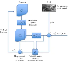
Figure 1.3: Schematic representation of the EnKF algorithm.

• Due to its formulation in terms of independent particles, it is embarassingly parallel.

1.5.1 Algorithm

Figure 1.3 shows a schematic diagram of the EnKF algorithm. Having an ensemble-based representation of the state in mind, consider an ensemble ofqinitially indepen-dent states sampled from a normal distribution with predefined mean and covariance matrix. The expected value of the system state corresponds to the ensemble average of these states

¯ xk =

1 q

q

Õ

j=1

x(_kj). (1.46)

Defining the scaled state perturbation matrix Ak as

Ak =

1 p

q−1[x

(1)

k −x¯k· · ·x (q)

k −x¯k], (1.47)

and the scaled output perturbation matrixH Ak(assuming the linearity of the

obser-vation function, i.e.,h(x)= H x) as

H Ak =

1 p

q−1

[y(_k1)−y¯k· · ·y (q)

(44)

where y(_kj) = h(x_k(j))and ¯yk is the ensemble average of the outputs, one can finally

compute the ensemble covariance matrix

Ck = Ak(Ak)T , (1.49)

which is an estimate of the state covariance matrix.

The filtering algorithm can be summarized as a succession of two steps: a forecast step (or dynamic update) and a analysis step (or measurement update).

Forecast Step

The state of each ensemble member at the next time step is estimated using the (possibly nonlinear) dynamic model (Eq. 1.18):

ˆ

x_k(j)₊₁= f(x_k(j),uk)+g(x (j) k )µ

(j)

k , (1.50)

where the hat is used to represent forecast variables. If applied to a linear system, this ensemble approach reduces the cost associated with the time-propagation of the state statistics fromO(n3)(classical KF) toO(n2q)(EnKF). Since typical ensemble sizes are no larger thanO(102), the overall cost is usually reduced by several orders of magnitude.

Analysis Step

The ensemble members are corrected in order to minimize the error with respect to the measurements in the presence of noise and model uncertainties. There are several paths that lead to the EnKF analysis formula. We here adopt the optimization approach by looking for the minimizer of the cost function

J(x)= 1

2kyk−H xk 2

R+

1

2 kx−xˆkk 2

ˆ

Ck

= 1

2[yk−H x]

T

R−1[yk−H x]+

1

2[x−xˆk]

T _ˆ

C−_k1[x−xˆk]. (1.51)

This optimization problem is then restricted to the affine space generated by the prior estimate of each of the ensemble members and the subspace spanned by the scaled perturbation matrix ˆAk. In other words, we look for a solution in the form

(45)

wherev ∈_Rq_{is the correction coefficient vector.}

After performing the proposed change of variables, we can restate the objective of the analysis step as finding

v= arg min v∈Rq

J(v) (1.53)

for each of the ensemble members, where

J(v)= 1 2kvk

2₊ 1

2kyk−Hxˆk−HAˆkvk 2

R. (1.54)

SinceJ(v)is quadratic inv, the solution is unique and corresponds to the root of

DJ(v)= v− (HAˆk)TR−1(yk −Hxˆk −HAˆkv)= 0 , (1.55)

which is given by

vk =

I +(HAˆk)TR−1(HAˆk)

−1

(HAˆk)TR−1(yk−Hxˆk) (1.56a)

=(HAˆk)T

R+(HAˆk)(HAˆk)T

−1

(yk −Hxˆk), (1.56b)

where we have used the Woodbury matrix identity to obtain the alternative solution. Notice that here we have the possibility to choose between performing the analysis in the ensemble space (q-by-qmatrix inversion - Eq. 1.57a), or in the measurement space (p-by-p matrix inversion - Eq. 1.57b), depending on which one is more advantageous[56]. In either case,q norp nsuch that an enormous reduction in computational expense is achieved compared to the KF/EKF.

The final solution is then obtained by projecting these coefficients back to the state space:

xk = xˆk + Aˆk

I +(HAˆk)TR−1(HAˆk)

−1

(HAˆk)TR−1(yk−Hxˆk) (1.57a)

= xˆk + Aˆk(HAˆk)T

R+(HAˆk)(HAˆk)T

−1

(yk−Hxˆk). (1.57b)

Algorithmically, when the inversion is done in the measurement space, instead of solving forvk, the representers’ formulation proposed by Evensen and Leeuwen [57]

is used:

R+(HAˆk)(HAˆk)T

bk =(yk−Hxˆk) (1.58a)

(46)

where the columns of ˆAk(HAˆk)T are called therepresentersand represent the

influ-ence vectors for each measurement. The vector bk then represents the magnitude

by which each of the representers actuates in ˆx.

For each ensemble member, yk must be independently sampled from a normal

distribution whose mean is the measurement vector obtained from the estimated system, and whose variance isRk. Due to this sampling step, this algorithm is often

referred to as perturbed observations (or stochastic) EnKF. Although this procedure introduces an additional sampling error, previous work by Lawson and Hansen [58] suggested it performs better in the presence of nonlinearities than deterministic alternatives.

It is worthy to note that one never needs to explicitly compute the covariance ˆCk

since it suffices to evaluate ˆAk(HAˆk)T and HAˆk(HAˆk)T. Both the Particle Filter

(PF) and the EnKF algorithms share the same forecast step, but their analysis steps are distinct. While in the PF the posterior PDF corresponds to a linear combination of the prior ensemble whose weights are calculated using the Bayes’ rule, the EnKF assign equal weights to all particles and correct the ensemble members themselves according to Kalman’s update rule[23]. Because the particles themselves are driven towards the measurements, the need for resampling is eliminated.

1.5.2 Initialization Scheme

In order to keep the cost at tractable levels, it is desirable to use ensemble sizes that are much smaller than the dimension of the state. Thus, being able to efficiently sample the initial ensemble plays a fundamental role in the filter performance. Therefore, following Evensen’s scheme[19]:

1. Using a long series of snapshots obtained from a long simulation of the phe-nomenon we are interested in, we build the data matrix ˆX = [x(1) x(2) · · · x(N)] and obtain the corresponding POD modes by computing the singular value decomposition

¯ x = 1

N ˆ

X1N×1 (1.59)

1 √

N−1

(Xˆ −x¯11×N)=UΣVT , (1.60)

(47)

2. In order to generateqindependent initial ensemble members, we restrict it to the subspace spanned by the firstqPOD modes:

A0= qr(r andn(q)) (1.61) X0=

p

q−1 ˜UqΣ˜qA0, (1.62)

where ˜Uq corresponds to the first q columns ofU, and ˜Σq is the upper-left

q × q submatrix of Σ. Here r andn(q) represents a q × q matrix whose entries where independently sampled from a zero-mean Gaussian distribution with unitary variance, andqr(·)correspond to an implementation of the QR decomposition.

A similar approach can be used to generate the ensemble of noise vectors needed to force the dynamics:

Ak = qr(r andn(q)) (1.63)

Mk = α

p

q−1 ˜UqΣ˜qAk , (1.64)

whereα is a parameter that controls the noise magnitude. In this case, the corre-sponding error covariance matrix is given byQ= α2U˜qΣ˜2qU˜qT.

1.5.3 Ensemble Size