GROVER : a graph plotting program for Sun workstations

http://wrap.warwick.ac.uk/

Original citation:

Chown, P. (1990) GROVER : a graph plotting program for Sun workstations. University of Warwick. Department of Computer Science. (Department of Computer Science Research Report). (Unpublished) CS-RR-162

Permanent WRAP url:

http://wrap.warwick.ac.uk/60857

Copyright and reuse:

The Warwick Research Archive Portal (WRAP) makes this work by researchers of the University of Warwick available open access under the following conditions. Copyright © and all moral rights to the version of the paper presented here belong to the individual author(s) and/or other copyright owners. To the extent reasonable and practicable the material made available in WRAP has been checked for eligibility before being made available.

Copies of full items can be used for personal research or study, educational, or not-for-profit purposes without prior permission or charge. Provided that the authors, title and full bibliographic details are credited, a hyperlink and/or URL is given for the original metadata page and the content is not changed in any way.

A note on versions:

The version presented in WRAP is the published version or, version of record, and may be cited as it appears here.For more information, please contact the WRAP Team at:

-Research

report

162

GROVER:

A

GRAPH PLOTTING PROGRAM

FOR SUN WORKSTATIONS

PAUL

CHOWN

VLSI

Architectures Group

(RR162)

The report is a manual for the GROVER plotting package, which provides a facility for users for a Sun Workstation to manipulate numerical data in graphical form. The interface to GROVER is in the form of an interpreted command language, allowing interactive manipulation of two dimensional graphs generated from a

variety of data formats. The interface can be operated from a standard character terminal although access !o a Sun workstation enables the effects of commands to be seen directlv.

Department of Computer Science University of Warwick

Coventry CV4 7AL

A

groph plotting

progrom for

Sun Workstotions

Poul

Chown

VLSI

Architectures

Group

ABSTRACT

This report is a manual for the CROVER plotting package, which provides a facility for users of a Sun Workstation to manipulate numerical data in graphical form. The interface to CROVER is in

the form

of

an interpreted command language, allowing

interactive manipulation of two dimensional graphs generated

from a variety of data formats. The interface can be operated from

3

3

4

5

5

6

6

8

17

3

4

t9 t9

21

B

b

zl

CONTENTS

Introduction

l.l

Bockground

1,2

Nototion

GROVER

documentotion

2.1

Invocotion

2.2

Environment Voriobles

2.3

Explonotion

of

Terms

Commond Longuoge

SunView Environment

Appendix A - Attributes

I

GlobolAttributes

2

Locol Aftributes

Appendix

B

-

Error Messoges

Appendix

C

-

Post Processors

GLASER

@nc

Introduclion

I

.l

- Bockground

GROVER was

written

in

the spring and

summer

of

7989

to

fill

a

need

within

the VLSI Architectures

Group

for

a tool

to plot

the

results of

simulations being carried

out

using the SPICE package. Since a reasonable

amount

of

time had

been

set

aside

for

this

project,

it

was decided

to implement a tool that

would allow

data samples to be plotted

in

a range of

styles

in

a flexible and interactive fashion.

The

plotting

requirements

for

a

number

of

measurements taken

at

the same time

from

a given system can be

fairly

complicated. For example a

SPICE simulation of a simple inverter

would

typically produce

two

sets

of

data, one

for

the

input signal and

one

for

the

output

signal.

For

the

remainder

of

this document,

it

\

rill

be assumed that the data consists

of

a

number of such 'sets'. Each

of

these sets

will

be referred to as a data 'trace'. To

return to

the inverter simulation, each measurement

in

a data trace is

represented by a pair

of

numerical values, one being a time value and the other a voltage value. As

well

as being able to produce a voltage-time plot

for

each

of

these 'traces'

it

would

be nice

to

be able

to

plot

one voltage

against

the other

to

obtain

a

voltage

transfer

curve

for

the

inverter

(assuming _that the simulation was a

low

frequency one).

It

was

with

this type of data manipulation

in

mind

that GROVER was written.

The

wide availability

of

Sun Workstations

within

the Computer Science

department made them a natural choice

for

the implementation

of

such a

tool.

Since

the

major

windowing

interface available

at

the time

was

SunView,

this

was chosen as the environment under

which

the package

would

be

implemented.

With

hindsight,

it

would

probably have

been more expedient

to

base

the

package

on

the XWindows environment as

this has gained more widespread acceptance.

A

future version of GROVER may include this upgrade.

Since

it

was written, GROVER has been

fairly well

used

within

the group

for

a variety

of

applications

and

has shown

that

the additional

effort

to

improve

flexibility

of

the

user interface was time

well

spent.

The

I ,2

-

Nototion

When

examples

of

program dialogue are

given within this

document, they

will

be printed using a Courier typeface such as :

This is an

example

Where an interaction between GROVER and a user

is

to be emphasized, the parts of the dialogue supplied by the user

will

be emboldened :

Do

you

realJ-y want to quit

?

y s

Parts

of

GROVER commands

and

parameters

that

are contained

within

the main body of the text

will

simply be emboldened.

F-:

UW@

Overview

This section describes the user interface

to

the GROVER

plotting

package

as it

is

currently

implemented

for

the Sun Workstation. The package is

intended

to

operate

primarily under

the

SunView windowing

environment

but

may

also

be

used effectively

from a dumb

terminal when

a

suitable

hard

copy device

is

available

to

produce the graphical

output. Sections

Two

and Three

_will

describe the user interface assuming

no

more functionality

than

that

available

from

a

standard

terminal.

Section Four

will

describe the additional features that are made available

by

the SunView interface

2,1

-

_Invocotion

The program is invoked from a UNIX shell

in

the standard way, by issuing a command

of

the

form

:

grover t -d I t -f file_name I

[data_file_name]

The program

will

then

initialise itself taking

advantage

of

the SunView

environment

if

such

is

available. Commands may be issued

to

GROVER

to

generate

a plot

or

multiple

plots, display

and manipulate them

in

a

SunView

window

(if

available)

md

save them to a file ready to be printed

on

a

laser

printer

or

plotter.

Commands

will

normally

be

typed

into

a character

oiented interpreter, although certain

common operations are

made available

through the

mouse

when running

GROVER

under

a

SunView

environment.

The

-d

argument

is

used

to

specify

that

a 'dumb' interaction

is

required

with

the

plotting

program i.e. no

plotting

canvas or corunand

window

are

to

be

generated even

if

the

program

is

running

under

SunView. This

mode

is

the only

mode available when the program

is running on

a

standard terminal, and so the -d option need not be given in that case.

The

-f file_name

option

is

used

to

specify a

file

from

which commands

can be read instead of reading them from the standard input device.

In

this

The last option,

data-file-name,

is

the name

of

the

file

from

which

trace data

is to

be read.

It

is not

absolutely necessary

to

specify

this on

the command line as data can also be loaded interactively

by

using GROVER commands

but

it

may be desirable when operating the package

in

a non-interactive mode. The data file formats that are acceptable by GROVER are

described in a later section.

2,2 - Environment

Voriobles

The GROVER package uses several environment variables

to

initialise

itself

and to locate certain special files. The values

of

these variables

will

need

to

be set

by

the

user

through

the

environment variable interface

provided by the login shell. This should be done before

running

GROVER.

The names of these variables and their functions are defined as follows :

GROVER_DIR

is

used

to

specify

an

initial

directory

for

GROVER to change

to

before entering the command interpreter.

If

no

value is

specifed then no directory change

will

take place.

GROVER_INIT

can

be

used

to

specify

a

start-up

file

of

GROVER commands that are to be executed before the command interpreter

is

made available

to

the

user.

This

start-up

file

may

contain any

valid

GROVER commands,

for

example

to

set

up

commonly used

macros or default plot settings.

GROVER_HELP

specifies

the

file

containing

help

information for

GROVER.

If

any

of

these environment variables are

not

defined when GROVER is invoked then no error

will

be produced, and no action

will

be taken. They are there

simply to allow

control

over

the program before the command interface becomes active.

2,3

- Explonotion of

Terms

The GROVER program

currently

obtains the data

to

be plotted

from

an

ASCII data

file

containing records of the form :

<name>

<fieldl>

<field2>

The name

of

the record

is

used

to group

the record together

into

traces,

each

of

which contains a set

of

information about a given data stream or

feature. The trace may be accessed

within

the package

by

specifying this

common name.

For

example

all

records

with

the

name

probel

may contain

two

fields

with

the

first field

containing the voltage value and the second containing

a

current value

for

a

given

point

in

time,

which

is

unspecified.

GROVER requires

that

all

data traces

in

the

input

have the same number

of fields, and that the attribute represented by each field be the same across

all

traces. Thus

if

trace 1,

field

1 represents time, then trace

2, field

L must also represent time.

It

may be the case that more fields are specified than

are required

by

any one data trace,

in

order

that

the above conditions be

satisfied.

If

this

is

the case then some fields

of

some data traces may be

filled with

zeroes (or any other meaningful value).

It

is a simple matter to

modify

GROVER so that

it will

accept data files in formats other than the one described here, and information on

how to

do this can be obtained

from

Paul Chown at the University

of

Warwick. The

current format has proved sufficient

to

satisfy

our

demands

on

the

program

but

other means

of

obtaining data may be

useful

(for

example

the direct

acceptance

of file

formats generated

by

other tools

such

as

SPICE).

Control over the format, layout

and axis

limiting

values

for

a

graph

is

accomplished

through

the

use

of

attributes,

each

of which is

used to control

a particular

feature

of

a plot.

There are

two

types

of

attributes,

global

attributes

which

define package-wide features (such as the number of fields in a record), and local attributes which define the characteristics of

the

individual plots

produced

by

the package.

Control over

attributes is

r:n

ll

lnrirArA

U UUU

\9\=

Commond

Longuqge

Control over the generation and manipulation of plots

within

GROVER is

achieved

through

the

use

of

a

command

language, assisted

in

the

SunView environment

by

use

of

the

mouse. The command language is

fairly

small

but

the use

of

such a structure allows

rapid

modification and

development

of

the

program.

Input

to

the

command

interpreter

may come

either

directly from the

user

(typing

commands

at

the

GROVER

prompt)

or

from

a

file. In

the

latter

case, the

file

being executed may be

either

a

start-up script,

a

complete

session

script (i.e

no

user

input

is

required throughout

the execution),

or

a

GROVER script

which

may be

invoked

from within

the

GROVER interpreter,

returning control

to

the user when the script has terminated.

As

has already been described,

plots within

GROVER are formed from

elements

of

the data traces that have been read from a data file. Once the

plot has been specified correctly,

it

becomes a member of a structure called the

plot list,

which contains the definitions

of

all

currently defined plots.

When the

plot is

created,

it

will

take

on a form

defined

by

the default

values of the

plot

attributes. These defaults may be set by the user through the command language. Once defined, the

plot

attributes become local to

that

plot

and may be

modified

independantly

of all

other plots. The

plot

that is being modified/examined is called the current

plot

and this may be changed as desired. Once a

plot

has been defined

it

can be saved to a

file

in

a

generic

form

ready

for

post

processors

to

produce device specific

plot

files.

The following

pages

contain

descriptions

of

the

commands

that

are

available to the user,

in

alphabetical

order.

Each entry specifies the syntax

of

the command and its arguments and is followed by a description

of

the action that is performed.

It

should be noted that the command language is

case Sensitive

-

all

commands

should be typed

in

lower

case unless otherwise specified.

ollplot

Produces one

plot for

each

of

the data traces

currently

held by GROVER Each

plot

produced makes use

of

the default attribute values

in

the same way as the

normal

plot

command. The use

of

this command is equivalent

to

typing

"plot

<tracename>"

for

every available data trace. When a large

number

of similar

traces are to be displayed as is often the case

with

VLSI

simulation results, the

allplot

command can save a

lot of

typing.

qllsqve

In

the sarne

way

as

allplot

will

produce a

plot for

every data trace

within

the system, allsave

will

produce a file for each

plot

containing a definition

of

that

plot

in

a device independant form. For each

plot,

the filename that

is

generated

by this

command is

of

the

form

"grv.<plotnum>". The

post-processing packages Ere

written

to look

specifically

for

filenames

of

this form.

qttribs

Produces a

list of

the attributes that are currently available

to

the user for

display and alteration using the show, set and

default

commands (q.v.).

The attributes are used to provide conkol over the layout and scaling of a

plot. Before any plots have been produced the list

will

consist solely of the

global attributes. When a

plot

has been defined, however, the

list

will

be

extended to include attributes local to the currently active plot. For a list of attributes and their functions please refer to Appendix A.

cleqr

Deletes

all

currently

defined plots and clears the

plotting

canvas without

deleting

the

data trace information

from

memory.

If

the data

trace information

is no

longer required and can also be deleted then the

flush

command (q.v.) can be used.

dqlq

Produces

a

list

of

the

data traces currently

held

in

memory. The names

given

by this

command are those recognised

by

the

plotting

commands

and should be referenced exactly as they appear.

If

no data is present when the command

is

issued then the message

"No

Data"

will

be displayed in

place of the list.

defoult <ottribute_nqme) = (velue>

Sets the default value

for

local attributes to the given value. The value set

by

this

command

is

the value

given

to

the attribute when a

new

plot

is

created. Subsequent modification

of

the local attribute

within

any

plot

will

not

affect

this default.

For

example,

to

superimpose

a

grid on

all

plots

created in future, issue the command :

default srid :

L

exec

<filenome>

Executes a

script containing

predefined GROVER commands as though they had been typed

in

at the keyboard. The exec command itself may not be used

from

within

a script

file

(i.e. recursively). The pathname

for

the

file

to be executed must be specified

if it

is not to be found

in

the current directory, as no search path mechanism has been implemented to date.

flush

Resets GROVER

to

a

state

almost as

though

it

had

just

been invoked

without

specifying

a data file.

All

data

and

plots

are

deleted

and

the

plotting

canvas is cleared. The default athibute values are

not

restored to

their original state, however.

In

addition to

this, the

file

specified

by

the

GROVER_INIT environment variable

is

not

re-executed when the

flush

command is issued. The

initialisation

file

can be re-executed

if

necessary

by using the exec command.

gofo

<plolnumber>

Set

the currently active

plot

to

be

<plotnumber>.

Each

plot

has

an identifying number

which

is displayed

in

the plot list. The

plot list

may be

displayed using the

list

command (q.v.).

lf

a new plot is defined then

it

is

appended

to

the end

of

the

plot list

and automatically becomes the new

aitive

plot. The active

plot is

the one whose local attributes are operated on

by

the various

attribute

manipulation commands.

help

Displays help

information

for

GROVER. The message that

is

displayed is

oUtiin-ea

from the

file

specified

by

the

GROVER-HELP environment

variable. The message

will

typicatly be a

list of

the available commands

and the attributes

that may

be accessed through them. The

help

facility

should be extend"ed to be more selective and to provide more detailed help

on

the use

of individual

commands. This has

not

been done

to

date as

there has not been suuficient demand to justify the work required.

FI

Lists

all

of

the currently defined plots

giving

an

identification

number for each

and

a

description

of

the

plot.

This description

is

given

using the

syntax

of

a complete

plot

command and

in

order

to

understand the plot description, the reader

is

referred

to

the

definition

of

that

command. A

typical entry

in

the

plot list

takes the following

form

:

t 1l -

v1,.2

vs v2.2 for all field

1

This example indicates that

tace

v1,

field

2

(field

2 is

in

this case voltage)

is

being

plotted

as the y-axis against the voltage

v2

as the x-axis

for

all common values

of

field

1 (in this case time). This example could therefore be specifying

a

Vin

vs.

Vout

plot for

a semiconductor device. When the

list is

displayed,

the currently

active

plot

is

indicated

_by

an

asterisk

immediately

to

the

left of its

identifying

number.

The

active

plot is

the plot whose local attributes are accessible to the user at that time.

lood

<filenome>

Loads a data

file

of

the given narne from disk.

If

data is already present in memory, then GROVER

will

interrogate the user to see

if that data may

be

overwritten.

A

'no'

reply

at

this

stage

will

leave

the

resident

data

untouched.

If

new

data

is

loaded then

all

of

the

old

data, and

any

plots

that were created _{using lhat} data,

will

be lost. This

is

because there is no

guarantee that the

two

sets of data are compatible and

allowing

them to be

loaded at the sarne time may cause confusion.

If

it

is necessary to produce graphs combining

fwo

sets

of

results

from different files

then this should

be

performed

under

LINIX

before

loading

the data

into

GROVER. By

performing this operation externally the meaning

of

the data can be taken

into

account

more readily.

The user should

be particularly

aware of

generating inconsistent data

-

for

example

combining

two

data

sets containing

time

information but having

different time origins or

units.

mocro

mocro delele

"mqcro'

mqcro

"mctcro'

₌

"€Xponsion'

Before user commands

are

passed

to

the GROVER

interpreter they

are

processed

by

an

elementary

macro pre-processor

which allows

simple

string substitutions

to

be performed. One possible use

of

this

facility

is to

specify more descriptive names for constants that are

in

regular use. As an

example the specification

of

a new plot requires that a specific

field

must be selected from a data trace

in

the following

way:

prcbel

.3

where

field 3

is

the

field

that

corresponds

to

the voltage value

of

the

particular

data trace

in

question. Using the macro pre-processor

we

can

define a macro

for

the

field

number:

ma:ro tvoltagerr-rr3rr

such that the above

field

specification may now be

written

in

a

far

clearer

way:

probel

.

voltage

Macros may be nested to 15 levels, but

it

not recommended that this many be used

in

practice as

it

will

beiome very

difficult

to keep track of exactly

what is meant on when a command is typed.

A

list of

all

currently defined macros may be obtained using the macro command on

its own.

A

macro

may be deleted using a corrunand of the form

macro

delete

"namet'

It

may be necessary

to

override the macro processor sometimes, protecting

particular

words

or

phrases

from

being

processed.

This

can

be

accomplished by surrounding the text by quotes, as given

in

the syntax for the macro command.

Although

not strictly necessary,

it

is

recommended that quotes be used

in

all macro commands as this

will

ensure that the text

is

not

expanded

before

the

command

is

executed. The use

of

quotes is absolutely necessary rr'hen using the macro delete command as without the quotes the name

rt'ill

be expanded and the command interpreter

will

see not the name

of

the macro

but

its expansion.

mqtch <plofnuml

_{= <Plotnum>}

Forces the axes

of

one

plot

to

be equal

to

those

of

another. This

is

used

where

a

particular region

of

one graph has been selected

and the

user

wants

to display the

corresponding region

of

another

graph.

It

is

also

useful to

unify

graphs on

which

the axes have been automatically scaled.

The

plot

on the

right

hand

side

of

the assignment statement

is

the one

used to provide the

new

scale, as

in

conventional assignment statements.

newponel

When

this

command

has

been implemented,

it

will

allow

additional

windows

to

be opened onto the

plotting

canvas

to

simultaneous viewing

of plots

that are located far apart.

At

the moment the

only

way to perform

direct

comparisons

of

plots that

are

far aprt

on

the

plotting

canvas

is

to

reproduce the two plots so that they then lie side by side, or to sent them to

a

hard

copy device. Should this facilty generate sufficient demand then

it

will

be implemented.

plol

<trqce>

(

vs

<lroce>

(

_foroll

<field>

_{) I}

Generates a new

plot

descriptor which

will

appear

in

the plot list as shown

by

the list command (q.v.). The local

plot

attributes

for

the new

plot

are

initialised

with

the current default attribute values.

If

the automatic axis

scaling algorithms are selected then they are called and the results used to

set

the

axis attributes. The

plot is

then sent

to

the canvas

window

if

the

package

is

operating under the SunView environment.

The

arguments

to

the

command

provide

a

complete description

of

the data

that is to

be

plotted

and require a small amount

of

explanation. In

order to generate a plot

it

is necessary to know the

following

information :

1) Which data is to be plotted along the Y axis. 2) Which data is to'be plotted along the X axis.

3) The

attribute

that these

two

sets

of

data have

in

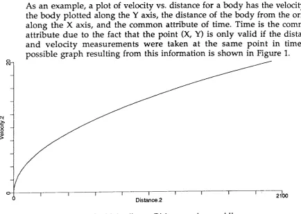
common that allow the X and Y data values to be paired.

As an example, a plot of velocity vs. distance

for

a body has the velocity of the

body plotted

along the Y axis, the distance

of

the body from the origin

along the

X

axis, and the common attribute

of

time. Time

is

the common

attribute due

to

the fact that the

point

(X, Y)

is

only valid

if the

distance

and velocity

measurements

were

taken

at

the

same

point

in

time.

A

possible graph resulting from this information is shown

in

Figure 1..

[image:15.595.87.522.459.768.2]

r3

A

plot is

specified

by giving

exactly this

information,

with

the package

filling in

information

fiom

default values

when

that information is

not

direily

specified

by

the user.

In

the above example,

fwo

data traces were available, Velocity

ind

Distance, each made up

of two fields

with

the first

representing

time

and the

second representing

the

value

of

the

relevant

attibute

at

lhat

time. The plot was produced by the command :

plot Velocity.2 vs Distance.2 forall

1

If

the default attributes are set correctly then

it

is possible to leave out the

majority

of

this

command

and

have

te

remainder

filled

in

from

the

default values.

In

this

wa!

r velocity and distance plots against time could

be produced

by

the

following

commands :

quit

Exits

from

the

GROVER package after asking

for

confirmation

from

the

user

that

the

session is

-really

terminated.

An

alternative

method

of

leaving

GROVER

is to

type

a

CTRL-D character

to

the

command interpreter,

indicating

that nb more input

is

available.

This

will

cause an

exit directiy

without-

querying

and so it

is

recommended

that

the

quit

command be used to avoid disasters'

rescole

Rescales the current

plot

using the default attribute values available at that

point

in

time. This iommand is

useful

for

restoring

the

grap,h

to

a

sane

state

after

a

number

of changes

have been

made,

although

since the current attribute values uru

tr"i,

the

plot

generated

may not

be identical

to

the

original.

The axis attributes are set

in

exactly _-the same manner as

they

wouia U"

had the

plot

just been created,

with

the

automatic scaling

algorithm being applied

if

necessary.

No

attributes

other

than the

axis attributes are changed.

sove

<Plot-id>

(

os <filenome>

)

saves

a

specified

plot to

a

file,

with

the filename being

gel-9r?t:d automaticuiiy

if

or,"

i,

not

supplie-d.- The.plot to be saved

is

specified by

specifying the

plot

_Ip

_.".*bLi

of

the

plot

in

the

plot

list

(see

the

list

cbmmand

for

more details)'

If

no filename is given

in

the command

line

then the output is placed

in

a

file

called

grv.0

in

the current directory.

Alternatively

a filename can be

specified using the as <filename> construct. The format

of

the output file

is

a PostScript description

of

the

plot

using a coordinate system from 0 to

1000

in

both

the

X

and

Y

directions.

It

is

envisaged

that

post-processing

filters

be used

to

group

plots

together

on

a page

and

set scale factors

/

colour

schemes

for

different devices. The PostScript

file

produced

by

the

save

command

does

not

therefore

contain

any

of

the

page

set

up commands that are norrnally required and cannot be sent directly to a laser

printer.

set <ottribule_nome>

_{= <flooting_volue>}

Assigns a specified value to either a local

or

a global attribute.

If

the name

supplied is

that

of

a local attribute and a

plot is

currently active then the

attribute

for

that plot only is altered. When a

plot

is created, the attributes

are

assigned

default

values.

In

order

to

change

this

default value

the

default

command (q.v.) should be used.

If

an attribute

is

changed that affects a particular plot (i.e a local attribute) then that plot

will

be redrawn

to

take

account

of

the

change.

All

properties

of

plots are

controlled

through

the use

of

attributes.

A

list of

the available attributes and their

functions

can

be found

in

the

relevant

appendix

at

the end

of this

document.

shift

<f

_loolin

g-vqlue>

Shifts

the

origin of

the x-axis

by

a

multiple

of

the range covered

by

the

complete x

ais.

The argument to this command is a signed floating point

value which

specifies

the

direction

and

amount

of

the

shift to

be

performed. The

origx

attribute is modified

by

adding the product

of

the

argument

and the x-axis range

to

it's original

value.

Although

the same operation can be achieved by modifying the attributes directly using the set

command,

shifting the graph

is

such

a

common

operation that

this command has been added as an accelerator. As an example of its operation

the

command

shift -0.1

will

shift

the

origin

1/10th

of

the current

x

range (i.e one graph division)

to

the left,

equivalent

to

shifting the graph

itself

to

the right

by

one

division.

show <qtlribule-nome>

Displays the current value of a particular attribute, as defined for the active

ptoi

if

the attribute is a local one. When operating under SunView mode

ihe

values

of

most attributes

will

be readily apparant,

but

when operating

without

a

windowing

interface

it

is

necessary

to explicitly

display

the attributes to see their values.

vshift

<flooting_volue>

Exactly

equivalent

to

the

shift

command,

but

acting

in

the

Y

(Vertical)

direction instead

of

the X direction.

vzoom

<flooling_vqlue>

Exactly

equivalent

to

the

zoom

command,

but

acting

in

the

Y

(Vertical)

direction instead

of

the X direction.

xlqbel

(

<new

lobel>

)

Allows the current

label

for

the

x

axis

to be displayed and

optionally altered.

The default

axis labelling consists

of

the name

of

the

trace from

which the

data was obtained and the

field

number

in

brackets. The trace

name is exactly as specified to the

plot

command. The

xlabel

command on its

own

will

display the current label. When followed

by

a character string

it will

change replace the old axis label by that string.

It

may be advisable to

enclose

the new

label

in

quotes

to

avoid macro expansions, and

to

allow

spaces to be

induded

in the label.

ylobel

(

<new

lobel>

)

Identical to the xlabel command, but operating on the

y

axis.

zoom

<flooting_volue>

Allows

the current

plot

to

be scaled

in

the

x

direction

with

the centre of the x-axis as the centre

of

scaling. This effectively allows the centre

of

the

graph

to

be magnified

or

reduced

in

the

x-direction

only.

The floating

point

value given

as the

only

parameter

is

the magnification factor, and

has a

minimum

value

of

0.1. The local attribute

step-x

is

divided by

this

value to obtain a new

step-x

value. Thus the command

zoom

2.0

will

enlarge

the

central

half

of

the

current

plot so that

it

occupies the entire

plotting

width.

Four

SunView

Environmenl

The user

environment under SunView

is

fairly

similar to

that

available

from

a

standard terminal,

the

same

command

driven

interface being provid.ed

through

a

window which

is

created

on

initialisation. However

iwo

additional

Ieafures are provided

-

a series

of

"accelerator" buttons to

sfeed

the

application

of

common oPerations,-

and a plotting

window

.r.,if,i.fr

_{displiysall of}

the plots

in

their

current form.

Commands may be

typed

"t

in"

terminal window

in

the manner that

has

already been

deicribed

in

previous sections.

Moving

the cursor to an accelerator button

and

clicking

bn

it

with

the

left

mouse

button

allows a

limited

number of

op"tutio",

"to

b"

carried

out

more

rapidly.

The following

accelerator

buttons are defined under the current version

of

GROVER :

quit

leave the GROVER environment, destroying the windows created

by

the

program

and returning

to

the system.-

-A-PoP-_up

window

will

appear to

confirm that this actioliis really desired before the system is aborted.

zoom

in

zoom

in

the current

plot

around the centre

line

of

the relevant axis. Two

zoom

in

buttons are provided, one

for

scaling _1n a horizontal direction (H)

and

the

other

for

the vertical

direction

(V)'

The axis

interval

and origin

are

automatically altered

to

perform the

desired scaling operation' This

button

performs'an operation-equivalent

to

the command

zoom 2

When this button

is

used

in

conjunction

with

the other

accelerator

buttons

there is a tendency

for

the

origin

and step values

for

the axes to

become

*or"

complex. For

this

reason it may be necessary

to

tidy

these

valuesupwhenthedesiredareahasbeenlocated.

zoom

ouf

the opposite action to zoom, so

zoom followed

by unzoom.should leave

the

active

plot

unaffected.

As

for

the

zoom

in

buttons'

there

are

two

buttons

for'this

operation

providing control

over both the horizontal and

vertical

directions'

L,R,U,D

allows

the graph to be moved

in

the direction corresponding to left, right, up

or

down

respectively. The buttons are arranged

in

a pattern to assist in

making

the correct selection. The operation that is actually performed is to

move the

origin

one tenth

of

the axis range

in

the opposite direction. This

gives the

impression

that the graph itself

is

moving

in

the

opposite

direction. Thus a

right

move is accomplished

by

moving

the

origin to

the

left

by

one step

unit.

The

origin

shifts

are implemented

using

the

shift

command

which

can be referenced

for

more information.

Plotting

Window

The

plotting

window

is

fairly

straightforward, being a

view

onto a colour canvas

on which

are drawn the current plots as specified

in

the

plot

list. When a new plot is created,

it

is allocated a new area of the canvas the size

of which

is defined by the globa! attributes

height

and

width.

The

plot

is

then

drawn into

this new area

of

the canvas. The creation

of

a new plot in

this way

may

well

mean

that the

canvas

must be

enlarged beyond the dimensions

of

the

window

in

which

it

is

drawn. Should this be the case,

the parts

of

the canvas that are not visible

in

the

window

may be brought

into view by

using

the scroll bars

that

are

provided at

the'edges

of

[tre

canvas

window.

The canvas

window

may also be resized

to

show larger

areas

of

the canvas or to allow different sized plots to be viewed in totality.

The mouse may be used to select a particular

plot from

the canvas window and make

it

the active plot, ready

for

manipulation using text commands

or

the

accelerator buttons. To select a particular

plot

simply

click the left

mouse

button within

the axes

of

the relevant

plot.

The 'active' indicator

in

the top

left

hand

corner

of

the

plot

should then be

illuminated,

indicating

that

it

has been activated.

This

light

will

always indicate the

currently active plot in the same way as the asterisk

in

the plot list.

Appendix

A

-

_Attributes

The attributes

within

GROVER are the means through

which

the user is

given control over the layout and

scaling

of

graphs produced

by

the package. The

following

pages

contain

a

list of

the

attributes available

through

the GROVER interface together

with

a description

of

the function

performed

by

each. The details

of

commands

that

may be

used

to

set

default and active values of these attributes are described

in

the Command Language definition of Section 3

of

this document.

The GROVER package has

two

types

of

attributes

that

can be accessed,

global

attributes

that

specify the

overall

attributes

of

the system and the data

on

which

it

is operating (number

of

fields per record etc.), and local

attributes that control plots on a local basis.

In

the latter case each defined

plot

has its own copy

of

the local attributes that may be different from the

copies of those attributes held by other plots.

I

-

_Globol

Athibutes

The global attributes define various default values that are used to control the formation of plots and to

inform

the package of particular system-wide values. They are

not

used

to

control

the

layout

of

each

plot but

are

still

necessary to define the environment

in

which

those plots are created. For this reason there is only one copy

of

each global attribute, the plots do not

contain copies

of

them as local values

would

have no significance. Thus the

defaultl for

global attributes are the same as the attributes themselves

and

so they may

be set

using either

the

default

command

or

the

set command

with

exactly the same meaning.

qulo_x

This

attribute determines whether

or not

the auto-scaling algorithm

is

to

be applied to the x axis when a

plot

is created. The auto-scaling algorithm examines the data being

plotted, and

uses the maximum and minimum

values that

it

finds

within

that data to calculate an approximate origin and

scaling factor for the axis along which that data is to be plotted.

The algorithm attempts

to

make the values that

it

chooses

for

the origin

and scale of the axis reasonable, i.e restricted to two significant figures. Due

to

numerical

inaccuracies

within

the

calculation

this

restriction

can

occasionally lead to some points not appearing on the graph or selection of a range that is larger than

it

needs to be (e.g a range of 5.1

for

data points

ranging from 0 to 5). This happens rarely and should not cause-a problem

o uto_y

This

is

the sister attribute

to

auto-x,

performing the

same operation for

the

y

axis.

Using

this

pair of

attributes

in

conjunction

with

locai defaults

for

origin

and

range values

allows

consistency between

plots

to

be

maintained even though a

wide disparity

in

data values may be present.

As

an example, the

following

commands specify that the

y

range

is

to be

from

0.0

to

5.0 (volts

in

this case),

with

the

x

axis being scaled

to

match whichever values are placed along

it

:

default origin_y :

0.0

default

range_y

:

5.0

3:f::1:

::i:-r

r

?

fields

Defines

the

number

of

fields

that each record

of

the

input file

contains (excluding the trace label at the start of each record). For example, to load a

data

file

with

records of the form

<name>

<fieldl>

<fie1d2>

<field3> <fie]d4>

the

fields

attribute should be given the value 4. The number of fields

in

a

record must

be

a

constant

for

any

particular

file,

it cannot change from

data trace to data trace or confusion

will

result when the file is read.

field_x

Specifies the data field that is plotted as the x-axis on the graph when a plot

is created. This value is used as a default to

fill

in

the information when

it

is

not

supplied directly

in

the plot command. By specifying a field number

within

the

plotting

command this value

is

superceded.

In

this

way

it

is

possible to specify only the data trace narne to be plotted,

with

this attribute

(in

conjunction

with

the

field-y

attribute)

defining

which fields are to be

plotted

on

which

axis. The

field-x

attribute also supplies the value for the common

data

field

required

by

the

plot

command.

In

this way

if

just

a

trace narne is supplied, then pairs of <x,y> values

will with

the values of x

being plotted

in

increasing order.

field_y

Specifies the data field that is to be plotted along the y axis

in

the same way

as the

field_x

attribute specifies the data

field

that is to be plotted along the

x axis.

height

Specifies the default height

of

the

plotting

area created for succeeding plot definitions as an integer number

of

pixels. Although the versions saved to

file

always use a conceptual

plotting

area

of

1000 by 1000 pixels, when the

plot

is actually drawn on the screen

it

usually occupies a smaller area,

with

perhaps a different aspect ratio.

The

height

attribute

is

used

in

conjunction

with

the

width

attribute

to specify the size and shape

of

that area

in

the canvas. When the package is being used

through a

standard

terminal

these attributes have

no

effect, since plots are not being

drawn to

a

plotting

canvas. These attributes also

have no effect once the plot has been save to a file as the size and shape

of

plots as they appear on an

output

device is defined by the post processor,

not by GROVER.

width

In

conjunction

with

the

height

attribute

already described

this

attribute

defines the area

of

the canvas that is to be used for new plots. The value of

the attribute is an integer number

of

pixels.

2

-

Locol Attributes

Local attributes are used to describe particular features of a plot, and so are not accessible

until

a plot has been defined. Before any plots are created

it

is

possible

to

set

up

the

default

values

for

the local attributes so

that

all

following

plot

creation commands

produce

acceptable

layouts.

The

defaults may be set

up

using

the

default

command as specified

in the

command

summary.

Once a

plot

has been defined the local variables for

that

plot

are allocated spave and initialised

with

the default values held by GROVER

at that point

in

time. the

local attribute

values

may

then be

modified

with

the

set

command

to

manipulate

the

graph. The

local attributes currently available are :

grid

a boolean flag that determines the presence

or

absence of a grid which can

be superimposed on the graph. When the grid is enabled, ten

low

intensity lines are placed across the graph

for

each axis, enabling the exact positions

of

points

on

that

graph

to

be

more

easily identified. The values

of

grid

used to enable or disable the grid are :

0 -

No

grid

1 -

Grid

linetype

specifies the type

of

mark that is to be used to indicate the data points on

the graph. The currently available modes are :

0

_-

cross

markers

I

:::*i";::;.:1""

The use

of

a continuous

line

to

mark

the data points means that a line is

drawn from point to point as ihey are placed on the graph. GROVER plots

the data points

by plotting

successively increasing values

of

the common data

field,

with

an <x/y> point being plotted

for

each common

field

value.

If

there is not a direct relationship between the x and

y

data values and the common data

field

then the graph

line

will

apparantly

leap

at

random

around the graph despite the fact that the points themselves may

lie

on a

uniform

curve. Under these conditions the graph should be plotted using

point

markers.

A

line that is drawn to a

point

outside the current axes

will

stop

at

the last

point

drawn

within

the axes, and

will

not be extended to

meet the edge

of

the plotting area.

origin_x,

origin_y

These two attributes locate the origin

of

the graph.

In

conjunction

with

the

step-x

and

step-y

attributes they define the scale and positioning

of

the

plot within

the x-y plane. The values assigned

to

the

origin

attributes are

floating

point

values. Note

that

the

origin

values may be altered

by

the

commands

that shift

and

scale

the

graph.

Under

the

SunView

environment

the numerical values

defining

the

axes are displayed

in

a

table to the right hand side of the graph itself.

slep_x,

step_y

In

order to completely specify the mapping between the x-y plane and the

graph that

is being plotted,

it

is

necessary

to

specify the position

of

the

origin

(using the

origin_x

and

origin-y

attributes) and the scales

of

the

two

axes. The axis scales are defined

by

the

step-x

and

step-y

attributes. Each axis

is divided

into

10

units to help

in

locating the positions

of

the points on the graph. The step attributes define the interval spanned by one

of

these units on the relevant

ais.

The range covered

by

the entire axis is

therefore L0 times the step attribute.

This convention is a

little

strange at

first,

but

it has been

found

that

it

is

more convenient

in

regular use than the specifying the range covered by the axis as a whole.

zero

Flag controtling the display of the two lines x=0 and _Y=0 on the graph

0 -

Do

not display zero lines

1 - ni qnl arz zafo lineS

L uLet'Lsl

Appendix

B

-

Error

Messoges

NON-FATAL

ERRORS

Cannot access

file

given when the program cannot access

or

create a file. This may be

due to non-existence

of

the

file,

a problem

with

access permissions,

or a larger problem

with

the system.

Line too long

an input

line

has

exceeded

the

limit

imposed

by

the

program

(probably around 255 characters).

Macro nesting too deep

The input line caused a macro expansion to be nested beyond

its

16

level

limit,

almost certainly due to a recursive macro or macro loop.

Macro expansion caused

line

overflow

The expansion of a macro has caused the line length to be exceeded.

No active

plot

a corunand has been issued that requires a

plot

to be active when none has been defined.

Syntax Error

This should never

really

appear as

it

is

too

blunt

and meaningless.

It

has been used as a temporary error message during development.

Macro does not exist

a macro operation has been invoked on a macro that does not exist.

This often appears when there are no quotes around a macro string.

Not running

under SunView

a command has been issued that requires the SunView interface to

be operational, and has found that

it

is not.

Athibute

does not exist

a corunand has been issued that has attempted to modify

or

access

an atrtibute that does not exist

within

the system

or

is not currently

active.

Field

limit

exceeded

the maximum number

of

fields

allowable

in

a

record

has been

exceeded.

It

is not possible to break the

limit

that has been compiled

into the _{Program using the}

fields

command.

Cannot open

file

A

command that needs to open a

file

has failed to open that file.

Unrecognized command : ....

A

command has been entered

that

GROVER does

not

recognise,

possibly due

to

macro expansion.

Invalid

plot

number

the

plot

number supplied

to

the

command does not correspond to any currently defined-plot.

Field number out of range

the field number supplied is too large/small.

Cannot

find

trace name

while trying

to seate a

plot,

the package could not

find

a data trace

with

the name that was supplied.

FAIAL

ERRORS

Invalid

operating mode

GROVER has entered

an

illegal

operating mode and has

had

to

abort

since

it

cannot

determine

what

environment

it

is

running

under. This indicates a major error

in

the code.

Invalid

GROVER_DIR value

The value

of

the environment variable

GROVER

DIR

cannot be

matched to a directory.

Invalid

GROVER-INIT value

The

value

of

the

environment

variable

GROVER

INIT

does not indicate a command file.

Usage : grover...

The

GROVER package has

failed

to

interpret the

command line arguments and tries to provide some hints for next time.

Cannot restore STDIN

probably indicates that a major system

limit

has been reached, such as the svstem

file

limit.

Out of Memory

The package has been told to load a large data file or generate many plots such that the system has

run

out of memory to store them.

Lexical Analyzer: ...

Another

error

message

that

indicates

a

major coding

error within

GROVER and so

will

almost certainly never apPear.

Appendix

C

-

Posf

Processors

Plot files generated using GROVER commands make use

of

the PostScript page layout language

to

record

point

and line

plotting

commands, colour

changes etc.

Within

each

plot file,

the graph is assumed to be plotted on a

page that has already been set up

with

axes running from 0 to 1000

in

each

of

the x and

y

directions.

No

page set up commands are contained

within

the plot files and so

it

is- not possible to send a

plot

file directly to the laser

printer

or

plotter. This

is

done

to

allow

simple post

processors

to

be

written that

convert

this

generic

format

into a

suitable

input

file for

a particular

output

device.

GROVER post processors are provided that take a number of plot files and

process them

in

a variety of ways to create a device specific plotting file. In this

way

it

is

possible

to

place a number

of

plots on

the same page and

perform

operations

such

as superimposing

plots

or

adding

page titles

without

having

to

regenerate

the plots using

GROVER

every

time

the

page layout is changed.

The remainder

of

this

appendix

will

contain manual pages

for

the

post processors that have currently been written

for

producing

plot

layouts for particular

output

devices. For each

of

these tools, a number

of

guidelines

are

provided

to

standardise

the

user interfaces between

tools,

and

to

simplify

their use :

Naming

Convention

The name

for

a post processor should consist of a 'g' followed by some sort

of

abbreviation

for

the

output

device that

it

is

wriiten

for.

For example'glaser'

or'ghpplot'.

Input

Files

Since

grover

generates

files

with

names

with

the

prefix 'gtt.',

invocation

of

a post processor should produce plots of all files of

that

form that

can be

found

in

the

current

directory,

in

more than one

output file

if

necessary.

Output Files

Output files from post processing programs should take the form

of

the

prefix 'plot.'

followed

by

an

integer

which

should correspond

to

the

input

file

that

was used

to

generate

it,

if

appropriate.

Arguments

Any

operation

differing

from

the standard

of

one

plot

per page

should be

selectable

through

options

only.

For

example, the

following options are suggested :

-h

provide help

information on

options.

-s

superimpose

the

plots

contained

within

the

input

files,

using the axis specifications

from

the

first

one

found

(i.e.

alphabetically

first

or

first

in

the filename list).

-t

"..."

put

the

title

that is contained

in

the following argument as a centred title across the top of the page

-n <plots>

put

a number

of

different plots on the same page, the

number

of

plots being supplied as <plots>. Put the plots on one above the other, rather than superimposed.

-x <xsixe> specify an x-size

for

the plots produced, given

in

cm.

Every plot produced

will

be this wide.

-y

<ysize> specify a

y size

for

the

plots

produced, as

in

the -x

option.

-p

<pagesize> specify the size

of

paper that the plots are

to

be

placed on (e.B

'A4','A3').

Additional

arguments that

do not

begin

with '-'

constitute a

list

of files that are to be plotted in place of the 'grv.' files.

GLASER

Documentotion

GLASER

is a

GROVER post-processor

to

convert generic

plot files into

page layout commands

for

an A4 Laser Printer. The syntax

for

the GLASER command

line is :

glaser

Ioptions]

filenames.

. .

If

filenames are not specified

in

the command line then GLASER

will

look

in

the current

working directory

to

locate

all

files beginning

with

the

prefix

'grv.'

and use those files to generate the Laser Printer files. The output consists

of

a number

of

files that

are

created

in

the

current directory,

generated

with

the

names 'plot.O',

'plot.l',

...

with

each

file

corresponding

to

one page

of

Laser Printer

output. The options supported

by

the current version are :

-h

lists

all

of

the current options

-n

<plots>

rather than

producing

output files

with

one graph

per page (the default), place <plots> graphs on a page before generating the next page.

-p

<size>

Change the page size to <siz,e> where <size> is specified as

the paper size name (e.9. 'A4','A3').

-s

superimpose

all

graphs that are placed on one page, using the axes obtained from the first graph plotted.

-t

<title>

place the

title

<title> centred at the top of each page.

-x <xdim>

-y

<ydim> Specify

the dimensions

of

the plots that are placed on the

page

(in

centimetres). The plots are normally scaled

to

fit

the paper that is available,

but

that scaling is overruled by these options.

As

an example

of

the use

of

GLASER, the

following

page was produced from a

directory

containing

four plot

files

with

the names

'9.r.0' to

'grv.3'. By issuing

the

command

glaser -t "barrout Simulation I4/B/89" -n

5

all four graphs are placed on the same page,scaled to

fit

one above the other, and

with

the specified

title at

the

top of

the page. The

output

was placed

in

a

file

called 'plot.O' which was then sent to the laser printer.

-.2

V(clk).1

V(int).1

-.2

V(Data). 1