Volume 7 - Article 8 | Pages 365–378

of peer-reviewed research and commentary in the population sciences published by the Max Planck Institute for Demographic Research Doberaner Strasse 114 · D-18057 Rostock · GERMANY www.demographic-research.org

DEMOGRAPHIC RESEARCH

VOLUME 7, ARTICLE 8, PAGES 365-378

PUBLISHED 15 AUGUST 2002

www.demographic-research.org/Volumes/Vol7/8/

DOI: 10.4054/DemRes.2002.7.8

Reflexion

Life Expectancy at Current Rates vs.

Current Conditions:

A Reflexion Stimulated by Bongaarts and

Feeney’s “How Long Do We Live?”

James W. Vaupel

1 Introduction 366

2 Heterogeneity in Frailty 366

3 Heterogeneity through Resuscitation 368

4 Empirical Examples 372

5 Conclusion 373

6 Acknowledgements 374

Notes 375

Reflexion

Life Expectancy at Current Rates vs. Current Conditions:

A Reflexion Stimulated by Bongaarts and Feeney’s

“How Long Do We Live?”

James W. Vaupel 1

Abstract

Life expectancy is overestimated if mortality is declining and underestimated if mortality is increasing. This is the fundamental claim made by Bongaarts and Feeney (2002) in their article "How Long Do We Live?", where they base their claim on arguments about "tempo effects on mortality".

This Reflexion explains why this claim is true in most heterogeneous populations. It suggests that demographers should be careful about distinguishing between life expectancy under current conditions, which is difficult and problematic to assess, and life expectancy at current rates, which can be estimated using standard methods. Finally, it speculates that there may be a deep connection between tempo and heterogeneity.

1 _{Director of Division 1 - Research Program on "Aging" and Head of the Laboratory of Survival and}

1. Introduction

Life expectancy is overestimated if mortality is declining and underestimated if mortality is increasing. The faster mortality is falling or rising, the more life expectancy is over or underestimated. This is the fundamental claim made by Bongaarts and Feeney (2002) in their article “How Long Do We Live?” (Note 1). They base their claim on arguments about “tempo effects on mortality”. Demographers who demand precise definitions, stochastic-process fundamentals and cogent proofs will not be persuaded by Bongaarts and Feeney’s loose analogies and sparkling intuitions. Their fundamental claim, however, can be shown to be correct, albeit from a radically different perspective and only if life expectancy is defined in a particular way. If life expectancy is defined as average age at death at current death rates, then life expectancy is simply calculated from the rates: there is no possibility of distortion. Life expectancy is defined, however, as “average age at death under current mortality conditions” by Bongaarts and Feeney as well as many other demographers. When death rates are changing, life expectancy calculated from current death rates will deviate from this life expectancy under current conditions in the way Bongaarts and Feeney claim in heterogeneous populations.

In this Reflexion I explain why Bongaarts and Feeney’s claim is true in most heterogeneous populations. I suggest that demographers should be careful about distinguishing between life expectancy under current conditions, which is difficult and problematic to assess, and life expectancy at current rates, which can be estimated using standard methods. Finally, I speculate that there may be a deep connection between tempo and heterogeneity.

2. Heterogeneity in Frailty

All populations are heterogeneous. Two individuals of the same age and sex in the same population can face very different chances of death. Some individuals are frailer than others and the frail tend to die first.

A simple but useful model of heterogeneity in frailty was developed almost a quarter of a century ago by Kenneth G. Manton, Eric Stallard and me (Vaupel, Manton, Stallard 1979). Let µ(x,y,z) be the force of mortality (hazard of death) for an individual of frailty z at age x and time y . Suppose

),

,

(

)

,

,

(

x

y

z

z

µ

o

x

y

where µo(x,y) is the “baseline” force of mortality for a “standard” individual of frailty one. Suppose

z

is Gamma distributed at age zero (which could be birth or some later

age after which the model is assumed to hold) with mean 1 and variance σ2. Then simple rearrangement of Vaupel, Manton and Stallard’s (1979) formula (11) yields

2

)

,

(

)

,

(

)

,

(

µ

σ

µ

x

y

=

o

x

y

s

_c

x

y

, (2)

where µ(x,y) is the force of mortality for the population and s_c(x,y) denotes cohort survivorship for the population:

∫

−

+

−

=

x

c

x

y

a

y

x

a

da

s

0

(

,

)

]

exp[

)

,

(

µ

. (3)

Note that µ(x,y) is a function of sc(x,y), whereas sc(x,y) is a function of the values of µ(a,y−x+a) for ages a up to x . Hence,

∫

−

+

−

=

_o x

da

a

x

y

a

y

x

y

x

0 2

].

)

,

(

exp[

)

,

(

)

,

(

µ

σ

µ

µ

(4)

This equation clearly indicates that the level of current population mortality at any age

after age zero is a function not only of current conditions, as captured by µo(x,y), but also of the historical mortality experience of the cohort.

Letµ~(x,y) be the force of mortality that would be suffered by a hypothetical cohort that lived under the mortality conditions prevailing at time y , as defined by

) , (x y

o

µ . Then, analogously to the result in (2), the frailty model implies

2

)

,

(

~

)

,

(

)

,

(

~

_µ

σ

µ

x

y

=

o

x

y

s

_p

x

y

, (5)

where period survivorship is given by

∫

−

=

x

p

x

y

a

y

da

s

0

(

,

)

~

exp[

)

,

(

~

_µ

_{. (6)}

2

)

,

(

)

,

(

~

)

,

(

)

,

(

~

σ

µ

µ

=

_



_



y

x

s

y

x

s

y

x

y

x

c p . (7)

To the extent that period survivorship is higher than cohort survivorship, the force of mortality under current mortality conditions, µ~ , will be higher than µ, the current force of mortality.

In Vaupel, Manton and Stallard (1979) a version of this formula is developed and applied to Swedish data. In 1975 Swedish female life expectancy at current death rates

was 78.15. If σ2 is 0.25, then the corresponding life expectancy under current conditions would be 77.52, almost eight months less. If σ2 is 1.0, then life expectancy falls to 76.36.

The Vaupel-Manton-Stallard frailty model is simplistic and the application to Swedish data is a special case. Nonetheless, the model and this application illustrate the general point. The current force of mortality at some age and time is a function of both current mortality conditions and the historical conditions that cohorts have experienced. A wide variety of other models of heterogeneous populations in which there are persistent differences among individuals in their age-specific susceptibility to death yield the same general conclusion (Vaupel and Yashin 1985; Yashin, Manton and Vaupel 1985; Vaupel, Yashin and Manton 1988). An individual’s frailty does not have to be fixed at birth but can change with age. Individuals can suffer debilitation, hormesis and recovery. To illustrate how general the basic result is, it is useful to consider another simple model.

3. Heterogeneity through Resuscitation

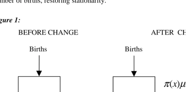
Anatoli Yashin and I developed a variety of simple, multi-state stochastic-process models for studying the impact of heterogeneity (Vaupel and Yashin 1986, 1987). Building on this line of thinking, a particularly simple variant of illustrative value can be developed as follows. Consider a population closed to migration that has experienced a constant mortality regime and a steady stream of Bbirths per year for more than a century. The age-distribution in such a stationary population will follow the lifetable survivorship pattern. And the size of such a population will simply be B times

the life expectancy e . Suppose at some instant of time the existing age-trajectory ofo mortality, described by µ(x), shifts as shown in Fig. 1. The idea is that a proportion

) (x

that these resuscitated individuals suffer some force of mortality µ+(x)at subsequent

ages that may be different from µ−(x). Also note that the population is no longer stationary after the change. The population will grow as the resuscitated population grows. Eventually, however, the annual number of deaths will balance the annual number of births, restoring stationarity.

Figure 1:

BEFORE CHANGE AFTER CHANGE

Births Births

The Resuscitated

π

(

x

)

µ

(

x

)

µ

(x

)

µ

−

(

x

)

=

(

1

−

π

(

x

))

µ

(

x

)

µ

+

(x

)

Before the mortality shift, life expectancy is e . Immediately following the shift,o period life expectancy at current death rates can be calculated from the values of

) (x

−

µ : call this life expectancy e .−

As the population of resuscitated individuals (in the right box of Fig. 1) builds up, the force of mortality for the entire population will be a weighted average of the forces of mortality in the two boxes. Let p(x,y)be the proportion of the population at age x

that is in the resuscitated box at time y after the mortality shift. Then the force of the

mortality for the entire population will be

) ( ) , ( ) ( )) , ( 1 ( ) ,

(x y = −p x y µ− x +p x y µ+ x

µ .

At any time y , life expectancy at current rates can be calculated using these values of

the force of mortality.

on the basis of the values of µ~ x( ). This life expectancy e~ is the mean length of life

experienced by all cohorts born after the mortality change. Hence, over the entire period from the time of the mortality change until the time when the new equilibrium is reached, life expectancy at current rates will differ from life expectancy under current conditions.

Consider a simple example. Suppose x e

x .1

00002 . )

( =

µ , which implies a life expectancy of about 79.4 years. Suppose π(x)=.5, all x , so that µ−_(x)=_.00001e.1x_.

For such a Gompertz trajectory life expectancy would be about 86.3 years. Finally, suppose µ+(x)=.5, all x . This constant hazard implies an expectation of life of 2 years. When the new equilibrium is reached, half the population will benefit from these extra two years of resuscitated life. The entire population will spend, on average, 79.4 years in the first box (because the hazard of exit from the first box is just µ(x).) Hence, in equilibrium life expectancy will be 79.4+(.5)(2)=80.4 years. In this simple example, then, life expectancy at current rates will jump from 79.4 to 86.3 years right after the mortality change and then will gradually decline to 80.4 years. Life expectancy under current conditions, however, will be 79.4 years before the change and 80.4 years at all times after the change.

In this simple example and in the general case as well, there are two changes. The

first is the immediate shift from µ(x)to µ−(x)and from e to o e . The second is the−

gradual change from µ−(x) to µ~ x( )and from e to the equilibrium life expectancy e~ .− If some people who would have died at age 0 can, under the new regime, endure to ω, the highest age attained, then equilibrium is reached after ω years. If no life is extended for more than

ε

years, then equilibrium is reached in

ε

years. A cohort of newborns born at the time of the mortality shift and all subsequent cohorts would experience the trajectory µ~ x( ) with average lifespan e~ . Hence, e~ is life expectancy

under current conditions whereas life expectancy at current rates gradually changes from e to e~ .−

In the simplest case, when µ+(x)=µ−(x) for all x , there is no effect due to

disequilibrium because the force of mortality is µ−(x)for both the resuscitated and those not rescued from demise. At all times after the mortality shift,

) , (x y

µ =µ−(x)=µ~ x( ).

cannot be restored to the level of more robust contemporaries not threatened with

imminent demise. Note that when µ+(x)=µ−(x) the resuscitated are not merely

restored to the old force of mortality µ(x): they benefit from the new, lower force of

mortality µ−(x). So this is pluperfect repair, more-than-perfect repair that incorporates mortality improvements.

If µ+(x)is bigger than µ−(x), which would be true in the reasonable case when the resuscitated are frailer than those not about to die, then there is both an immediate

shift and a lingering disequilibrium effect. If the values ofµ+(x)are large, then the mortality decline will not increase equilibrium life expectancy very much—and equilibrium will be approached quickly. The disequilibrium effect will be almost as big as the shift effect and of the opposite sign. The shift effect will be negative and could be considered to be a distortion because it will appear as if mortality has considerably declined. The positive disequilibrium effect will offset this.

There may be some cases, however, when µ+(x)is smaller than µ−(x). Suppose that the population is heterogeneous and that the mortality improvement mostly helps the robust rather than the frail. This could be the case for a population with subpopulations of men and women; smokers and non-smokers; rich, educated people and poor, uneducated people. If health progress largely helped women, non-smokers, or the well-off, then the resuscitated might enjoy better life chances than the average non-resuscitated person. In this case, the shift effect would be negative and the

disequilibrium effect would also be negative. Life expectancy e would be longer than−

o

e and e~ would be longer than e .−

In general, regardless of whether µ+(x)is bigger or smaller than µ−(x), the shift effect results in a discrepancy between life expectancy at current rates and life expectancy under current conditions. The size of this discrepancy depends on the extent to which the mortality change puts the population in a disequilibrium in which the current age-trajectory of mortality is different from the trajectory in equilibrium. There is “mortality momentum” as age-specific death rates move towards their equilibrium levels. This momentum can be viewed as being a consequence of the changing composition of the population, i.e., changing heterogeneity.

acquired or revealed by resuscitation. When mortality is increasing, Fig. 1 cannot be used but two kinds of people can still be distinguished. There are people who will die now who would otherwise have died later. And there are people who will not die now.

For simplicity, consider the case of declining mortality as illustrated by Fig. 1. Before the mortality change, everyone is in the same box. Just after the change, resuscitated individuals start flowing into the right box. To begin with, the population in this box is zero but this population gradually builds up to an equilibrium level. In equilibrium, the inflow of people into the box is counterbalanced by the outflow of deaths from the box. The people in the second box have different life chances than

people in the first box, as long as µ+(x)≠µ−(x)for at least some ages x. That is, the population is heterogeneous. Furthermore, the degree of heterogeneity right after the mortality shift is different from the degree of heterogeneity in equilibrium. This heterogeneity and the change in it produces the difference between life expectancy under current conditions and life expectancy at current rates.

The above discussion focuses on a very simple case in which there is a one-time mortality shift. It can be generalized to more realistic situations in which mortality is changing continuously over time. It can also be generalized in other ways. For instance, the force of mortality for the resuscitated could depend not only on age but also on time since resuscitation and on the heterogeneous structure of the population with regard to various risk factors.

4. Empirical Examples

5. Conclusion

The Vaupel-Manton-Stallard frailty model, the Vaupel-Yashin resuscitation model and these empirical examples illustrate the general point. If (1) cohort survivorship to some age is different from the survivorship that would be experienced by a hypothetical cohort living under current mortality conditions and (2) the level of survivorship to that age influences the composition of individuals at that age with regard to their chances of death, then the current force of mortality, µ, will differ from µ~ , the force of mortality that would be observed in a cohort that lived under current mortality conditions. Hence, life expectancy under current mortality conditions, calculated using central death rates or probabilities of death related to µ~ , will differ from life expectancy at current mortality rates, calculated using central death rates or probabilities of death related toµ. The more current conditions differ from historic conditions, the more life expectancy under current conditions will differ from life expectancy at current rates. The difference depends on the action of selection (i.e., the differential survival of the frail), debilitation, hormesis, and changing risk factors: different models will yield different estimates. As illustrated above, if mortality is declining life expectancy under current conditions can be higher than life expectancy at current rates, in some kinds of special circumstances. Under a wide variety of plausible conditions, however, Bongaarts and Feeney’s opposite claim will hold.

Bongaarts and Feeney propose an alternative measure of life expectancy that corrects for “tempo distortions”. Is their measure a better indicator of current mortality conditions? This is a difficult question that requires careful definitions, meticulous analysis, and rigorous mathematics based on probabilistic underpinnings. John Bongaarts has told me that he believes that tempo and heterogeneity are completely different concepts and that tempo effects can distort mortality in homogeneous populations. He may be right about this. Other scholars have told me that they think the notion of tempo effects on mortality is a red herring, a pink elephant, a bête noire, a siren’s song. They may be right about this. My conjecture is that there may turn out to be a deep relationship between “tempo distortions of mortality”—when that concept is clearly defined—and heterogeneity, probably of the acquired or revealed sort in resuscitation models. Anatoli Yashin and I have begun to try to think about this. We are not at all sure, however, that this duality will turn out to be a valid, useful notion. How best to assess the level of mortality under current conditions is an intriguing, puzzling question for demographers to ponder, a question at the historic core of demography.

6. Acknowledgements

Notes

1. In an email to me on April 2, 2002, John Bongaarts wrote: “The key insight from the BF paper is … that e0 is a function of the rate of change in the mean age at

death.”

References

Avdeev, A., A. Blum, S. Zakharov and E. Andreev (1998) “The Reactions of a Heterogeneous Population to Perturbation”, Population: An English Selection 10: 267-302.

Bongaarts, J. and G. Feeney (2002) “How Long Do We Live?”, Population and Development Review 28(1): 13-29.

Khazaeli, A.A., L. Xiu and J.W. Curtsinger (1995) “Stress Experiments as a Means of Investigating Age-Specific Mortality in Drosophila Melanogaster”, Experimental Gerontology 30: 177-184.

Livi Bacci, M. (2000) “Mortality Crises in Historical Perspective: The European Experience” pp. 38-58 in G.A. Gornia and R. Pannicia (ed.) The Mortality Crisis in Transitional Economies, Oxford University Press: Oxford.

Oeppen, J. and J.W. Vaupel (2002) “Broken Limits to Life Expectancy”, Science 296: 1029-1031, available online at http://www.demogr.mpg.de/publications/ files/brokenlimits.htm .

Shkolnikov, V.M. and G.A. Cornia (2000) “Population Crisis and Rising Mortality in Transitional Russia”, pp. 253-279 in G.A. Cornia and R. Pannicia (ed.), The Mortality Crisis in Transitional Economies, Oxford University Press: Oxford.

Vaupel, J.W. (1986) “How Change in Age-specific Mortality Affects Life Expectancy”, Population Studies 40:147-157.

Vaupel, J.W. and V. Canudas Romo (2000) “How Mortality Improvement Increases Population Growth” pp. 345-352 in E.J. Dockner et al. (eds.), Optimization, Dynamics and Economic Analysis: Essays in Honor of Gustav Feichtinger, Physica Verlag: Heidelberg, also available at http://www. demogr.mpg.de/Papers/Working/wp-1999-015.pdf.

Vaupel, J.W., K.G. Manton and E. Stallard (1979) “The Impact of Heterogeneity in Individual Frailty on the Dynamics of Mortality”, Demography 16: 439-454.

Vaupel, J.W. and A.I. Yashin (1985) “Heterogeneity’s Ruses”, The American Statistician 39: 176-185.

Vaupel, J.W. and A.I. Yashin (1987) “Repeated Resuscitation: How Lifesaving Alters Life Tables”, Demography 24: 123-135.

Vaupel, J.W., A.I. Yashin and K.G. Manton (1988) “Debilitation’s Aftermath: Stochastic Process Models of Mortality”, Mathematical Population Studies 1: 21-48.

White, K.M. (2002) “Longevity Advances in High-Income Countries, 1955-96”, Population and Development Review 28(1): 59-76.

Yashin, A.I., J.W. Cypser, T.E. Johnson, A.I. Michalski, S.I. Boyko and V.N. Novoseltsev (2002). “Heat shock changes heterogeneity distribution in population of Caenorhabditis Elegans: Does it tell us anything about biological mechanism of stress response?”, Journal of Gerontology: Biological Sciences 57A: B83-B92.